|
|
|
MEMP Homepage |
MEMP Phase I Final Report
|
Table of Contents
Table of Figures
Table of Tables
Glossary
1. Introduction
1.1. Background
1.2. Environmental Impacts of Nonpoint Source Pollution
2. Scientific Concepts
2.1. The Hydrologic Cycle
2.1.1. Description
2.1.2. The SCS-CN method
2.1.3. Curve Number Identification from Rainfall Runoff Records
2.1.3.1. CN determination for a single event
2.1.3.2. Determining catchment curve number from multiple events
2.1.3.2.1. The average curve number approach
2.1.3.2.2. The Hawkins-Hejlmfelt-Zevenbergen (HHZ) approach
2.1.3.2.3. The frequency-matching technique.
2.1.4. Estimating CNs from Handbooks for Ungaged Catchments
2.2 Water Erosion Processes
2.2.1. General Description
2.2.2. The Universal Soil Loss Equation (USLE)
2.2.3. Computation of USLE Factors
2.2.3.1. R, the rainfall-runoff erosivity index
2.2.3.2. K, the soil-erodibility factor
2.2.3.3. LS, the topographic factor
2.2.3.4. C, the crop-management factor:
2.2.3.5. P, the conservation-practice factor:
2.2.4. Nutrients and Chemical Loading
3. Results of the Data Collection Experiments
3.1. Study Site Description:
3.2. Rainfall Data
3.3. Conversion of Units and Data Correction
3.3.1. Runoff Measurements
3.3.2. Concentration of Chemicals and Sediments
3.4. Data Adjustment and Quality Monitoring
3.4.1. Data Adjustment
3.4.2. Data Quality:
4. Data Analysis
4.1. The Runoff Record and Rainfall-Runoff Relationships
4.2. Water-Quality Data Analysis
4.2.1. Introduction
4.2.2. A Comparison of Crops and Crop Management Practices
4.2.2.1. Total Dissolved Solids (TDS)
4.2.2.2. Oxidized Sulfate (SO4)
4.2.2.3. Nitrate (NO3)
4.2.2.4. Orthophosphate (PO4)
4.2.2.5. Other dissolved salts: Sodium (Na) and Potassium (K)
4.2.2.6. Soil loss (Sed.)
5. A Simple Method for Multiple-Objective Evaluation (MOE)
6. Recommendations
6.1. Recommendations Regarding Experimental Infrastructure
6.1.1. Runoff Collection Pits
6.1.2. Contributing Area
6.1.3. Raingages
6.1.4. Rainfall Intensity
6.2. Recommendations Regarding Data, Reporting, and Documentation
6.2.1. Nutrient Application Data
6.2.2. Full Reporting of Rainfall Events
6.2.3. Soils Data
6.2.4. Promptness, Initial Analysis, and Feedback
6.3. Future Directions
7. References
Table of Figures
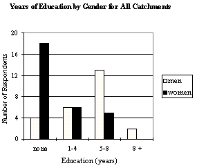
1. Locations of MEMP monitoring sites
2. The main components of the hydrologic cycle as applied to a representative column of soil
3. The SCS curve number relationship
4. Example of the rainfall-runoff relationship for Pit #1
5. A photographic sequence illustrating the impact of raindrop splash
6. Schematic diagram of the USLE standard plot used to determine K, the soil-erodibility factor
7. Break-point and hyetograph plots of a hypothetical storm for use in computing EI
7. The USDA soil texture triangle
8. The topographic factor LS for different slopes and slope lengths
9. Schematic representation of the effect of surface cover on soil erosion
10. The nitrogen cycle within the soil-plant-atmosphere system
11. Plant response to nutrient availability
12. The drainage system of Malawi
13. Actual locations of the field pits relative to one another in Chilindamaji Watershed
14. Schematics of field plots/pits and erosion-control plots
15. Daily precipitation time-series for Chilindamaji Watershed
16. Total monthly precipitation for Chilindamaji Watershed
17. Conceptual framework for runoff depth-adjustment
18. Comparison between monthly and total runoff values for different farm management systems in Chilindamaji Watershed
19. Rainfall-runoff relationships for the four field plots and the three erosion-control plots in Chilindamaji Watershed, January � April, 1995
20. A comparison of rainfall-runoff relationships between traditional cropping systems and management systems that aim to control erosion
21. Monthly and seasonal TDS losses from field and erosion-control plots in Chilindamaji Watershed
22. Monthly and seasonal SO4 losses from field and erosion-control plots in Chilindamaji Watershed
23. Monthly and seasonal NO3 losses from field and erosion-control plots in Chilindamaji Watershed
24. Monthly and seasonal PO4 losses from field and erosion-control plots in Chilindamaji Watershed
25. Monthly and seasonal Na losses from field and erosion-control plots in Chilindamaji Watershed
26. Monthly and seasonal K losses from field and erosion-control plots in Chilindamaji Watershed
27. Sediment yields based on the partial elimination method
28. Sediment yields based on the filtered sample
Table of Tables
1. Sample CN calculations from a single rainfall-runoff event
2. An example average CN computation
3. Sample calculation of catchment CN using the HHZ approach
4. Soil hydrologic groups classified according to saturated hydraulic conductivity
5. Identification of Antecedent Moisture Conditions
6. Handbook CN Identification
8. Steps in the Calculation of Total Storm Energy, EI
9. K factors computed for average soil properties for USDA soil texture classes
10. Saturated hydraulic conductivity, permeability class, and hydrologic group of major USDA soil texture classes
11. List of the USLE crop-management factor C during different stages of various cropping cycles
Explanation of terms
12. P for various slopes and maximum slope lengths
13. Configuration of field pits and erosion-control plots in Chilindamaji Watershed
14. Excluded runoff events, Chilindamaji Watershed, Jan. - Apr., 1995
15. Water-quality parameters for included events, Chilindamaji Watershed, Jan. - Apr., 1995
Pit #1 (Burley tobacco)
Pit #4 (Burley tobacco)
Pit #2 (Maize)
Pit #3 (Maize)
Control Plot #1 (Burley tobacco)
Control Plot #2 (Fallow)
Control Plot #3 (Maize)
16. Demonstration of a simple MOE for the Chilindamaji Watershed
|
abstract |
I + C |
|
BOD |
Biological Oxygen Demand. |
|
C |
The amount of rainfall intercepted by plants. |
|
CN |
The curve number coefficient in the SCS-CN method. |
|
CNe |
The estimated average curve number. |
|
CNi |
The computed curve number for the ith runoff producing event. |
|
EPA |
United States Environmental Protection Agency. |
|
ET |
Evapotranspiration. |
|
HHZ |
The Hawkins-Hejlmfelt-Zevenbergen approach for estimating CNs. |
|
i |
The rainfall event (storm) counter. |
|
I |
Water infiltration into soil. |
|
I a |
The initial abstraction |
|
MEMP |
Malawi Environmental Monitoring Program. |
|
MoREA |
Ministry of Research and Environmental Affairs. |
|
n |
The total number of runoff producing events. |
|
NPSP |
Nonpoint Source Pollution. |
|
P |
Precipitation (for conditions in Malawi, equivalent to rainfall). |
|
P e |
Deep percolation into soil. |
|
PSP |
Point Source Pollution. |
|
Q |
The total daily runoff volume. |
|
Qe i |
The estimated runoff for each rainfall event. |
|
R |
Surface runoff. |
|
S |
Soil water storage |
|
S |
The maximum potential difference between P and Q at the beginning of a storm. |
|
SCS-CN |
The U.S. Soil Conservation Service Curve Number method. |
|
S e |
Estimated soil water storage. |
|
S i |
Lateral subsurface inflow into soil. |
|
SM |
Soil moisture. |
|
S o |
Lateral subsurface outflow from soil. |
|
USAID |
United States Agency for International Development. |
|
AMC |
Antecedent moisture conditions. |
|
USDA |
United States Department of Agriculture. |
|
USLE |
The Universal Soil Loss Equation. |
|
A |
The USLE sediment yield. |
|
R |
The USLE rainfall-runoff erosivity index. |
|
K |
The USLE soil-erodibility factor. |
|
L |
The USLE length-of-slope factor. |
|
S |
The USLE degree-of-slope factor. |
|
C |
The USLE crop-management factor. |
|
P |
The USLE conservation-practice factor. |
|
em |
The kinetic energy of the mth intensity period for a unit rainfall. |
|
im |
The rainfall intensity period energy. |
|
Em |
The total kinetic energy for the intensity period. |
|
I 30 |
The maximum 30-minute rainfall intensity. |
|
EI |
The total kinetic energy of a storm. |
|
im |
The rainfall intensity for the mth period. |
|
Pem |
The cumulative rainfall at the end of the mth period. |
|
Psm |
The cumulative rainfall at the start of the mth period. |
|
tem |
The time at the end of the mth period. |
|
tsm |
The time at the start of mth period. |
|
a |
Percent soil organic matter |
|
b |
The soil structure code. |
|
c |
The soil profile permeability class. |
|
SF |
The soil structure factor. |
|
TF |
The soil texture factor. |
|
PF |
The soil permeability factor. |
|
M |
The soil texture parameter. |
|
l |
The slope length. |
|
q |
The slope angle. |
|
m |
The slope steepness parameter. |
|
SPHA |
The soil-plant-hydrosphere-atmosphere system. |
|
|
The ith event running average storage parameter. |
|
Sj |
The jth event storage parameter. |
|
MOE |
A Multiple-Objective Evaluation. |
|
Sed. |
Soil sediment loss. |
|
TDS |
Total Dissolved Solids |
|
WQDSS |
The USDA Water Quality Decision Support System. |
The United Sates Agency for International Development [USAID] and the government of Malawi are collaborating to provide the Malawi Environmental Monitoring Program [MEMP] with the necessary field, technical, and analytical training to carry out several environmental monitoring activities. MEMP was initiated to fulfill a threefold mission aimed at assisting the Ministry of Research and Environmental Affairs [MoREA] and other departments to:
1.Monitor the environmental impacts of policy reforms, in particular the impacts of smallholders' production of burley tobacco;
2.Establish a national capability to assess, monitor, and manage the environmental resources of Malawi; and
3.Provide equipment, training, and methods necessary for the fast and efficient production of maps, documents, and reports based on the results of MEMP's environmental monitoring activities.
To fulfill the above objectives, MEMP has been conducting monitoring programs in five small catchments near Nkhata Bay, Chikwawa, Dowa, Mangochi, and Kassungu (Figure 1). The monitoring activities include water sampling at catchment outlets, installation of erosion control-plots and pits, field monitoring pits, and the installation of automated samplers at two of the above-mentioned locations.
Although MEMP is a newly established program, it has the potential to become an integral part of the decisionmaking process at the level of national agricultural policy as well as at the level of operational farm-management. MEMP's capabilities can be enhanced through a combination of well-planned pilot data collection campaigns, training activities, scientific collaborations, and publications.
Providing the necessary training in the area of evaluating the environmental impacts of farm practices is at the heart of MEMP's objectives, and this report represents an effort in that direction. However, because the existing environmental record is too short to comprehensively evaluate and characterize the environmental impacts of different practices, this report concentrates on establishing guidelines for data analysis rather than providing policy recommendations. The report will attempt to make maximum use of the data collected from several erosion control-plots and field pits for the purpose of illustrating procedures such as (a) the identification of empirical rainfall-runoff relationships, (b) quality control and reduction of data, and (c) statistical analyses. Scientific and conceptual principals will be briefly illustrated, emphasizing operational aspects such as unit conversion, criteria-based selection of acceptable datasets, and data requirements for different environmental assessment objectives.
1.2. Environmental Impacts of Nonpoint Source Pollution
Environmental pollution of surface and ground water resources is classified as being either point source pollution [PSP] or nonpoint source pollution [NPSP]. PSP is defined as a concentrated effluent discharge at a given point. Examples of PSP include leakage from fuel tanks into groundwater, sewage effluent discharge into a lake or a stream, and other identifiable and usually measurable sources. On the other hand, NPSP is associated with the natural transport of dissolved and suspended materials carried by overland flow of storm water and/or irrigation water into streams and within porous soils. Major sources of NPSP include sediment, nutrients, pesticides, carbonaceous biological oxygen demand [BOD], nitrogenous BOD, and pathogens.

Figure 1. Map of Malawi depicting the locations of MEMP monitoring sites. Note that the sites are distributed in all three regions of the country (north, central, and south).
Transport and loading of nonpoint source pollutants have been occurring since geological times due to natural processes. However, transport and loading rates can be accelerated or decelerated by human activities that modify the natural properties of the watershed, thereby affecting the driving processes. Countless examples of the impacts of agricultural activities on the rate of erosion, nutrient loading, and pesticide loading can be found around the world. In 1991, The United States Environmental Protection Agency [EPA] has identified agriculturally-derived NPSP loading into surface water as the major cause of river and stream impairment in the continental U.S. In Malawi, erosion-caused siltation has reduced the effective head above the turbine from 6 m to 3 m in the Lower Shire River. Whether agricultural activities are responsible for the erosion can only be answered by quantifying and comparing the rate of erosion from different management systems.
Soil and nutrient losses have both on-site and off-site impacts. On-site impacts exist within the boundary of the field and/or the watershed, and include loss of productivity, soil degradation, and increased salinity. The economic loss associated with these impacts can be very high. For example, Pimental et al. (1995) reported that an estimated 4 billion tons of soil are lost from U.S. cropland each year. Furthermore, an estimated 1 million ha of cropland are lost each year in developing nations. The cost of associated on-site nutrient losses in the U.S. reaches $20 billion/year; another $7 billion/year is the estimated cost of lost soil.
Off-site impacts represent the consequences of (a) runoff mediated sediment discharge, nutrient loading, and pesticides loading of surface streams, and (b) chemical loading of groundwater via infiltration and deep percolation. Eutrophication of surface-water bodies is the most critical off-site impact of nutrient transport, and occurs as a direct result of excessive nutrient concentrations in the water body. Eutrophication significantly reduces dissolved oxygen, and eventually leads to the extinction of aquatic life in the water body. In addition to the degradation of water quality, the deposition of sediments can lead to the reduction of water storage capacities in watercourses and reservoirs. Termed "stream siltation," this can (a) cause an increase in the frequency and magnitude of floods, and (b) blanket the stream-bottom gravel beds necessary for the reproduction of some fish species.
Because of the significant adverse economic and environmental impacts of NPSP as well as the high costs of erosion control and abatement, selecting environmentally sound � yet profitable � farm-management practices is inherently a multiple-objective decisionmaking problem. Policymakers must have access to accurate and sufficient information regarding the various environmental impacts of existing and proposed agricultural management systems. This report aims to provide MEMP staff with the tools to improve the accuracy of the information conveyed both to policymakers and to those scientists who may be interested in analyzing the information contained in current or future datasets.
Informed agricultural policy decisions must be based on sound technical advice. Technicians, scientists, and farmers need to attain a close level of cooperation to ensure successful culmination of organized experimental studies and data collection campaigns. Furthermore, technical personnel need to be familiar with the basic scientific concepts underlying experimental studies. Such familiarity is an invaluable asset to any environmental monitoring program, because it equips project personnel with the necessary skills to:
1.Monitor the quality of data,
2.Take scientifically-based actions,
3.Perform initial data analyses with potential uses of the data in mind,
4.Be able to work within interdisciplinary teams; and above all,
5.Communicate these concepts to farmers.
To aid readers in attaining familiarity with these basic scientific concepts, Section 2 provides a brief description of the hydrologic cycle, erosion and sedimentation processes, and the nutrient cycle from an agricultural perspective. Detailed technical discussions are avoided whenever possible without compromising the quality of the information provided.
As mentioned in Section 1.2, nonpoint source pollutants are suspended and dissolved materials carried by storm water over the land, into streams, and within the porous media of the soil. Clearly, water acts as the detaching agent of soil particles, dissolving agent of chemicals, and a transport agent of suspended and dissolved materials. It is imperative, therefore, to develop an understanding of the hydrologic cycle.
There are several possible conceptual models of the hydrologic cycle. These models are scale dependent and reflect the dominant hydrologic processes at that scale and for a specific situation. In this report, we focus on the agricultural aspects of the hydrologic cycle. Figure 2 is a schematic diagram of the components of the hydrologic cycle for agricultural lands.

Figure 2. Simplified diagram of the main components of the hydrologic cycle as applied to a representative column of soil. Note that infiltration is an output from the surface component as well as an input to the soil component of the cycle.
Figure 2 provides guidance for constructing a version of the conservation of mass equation. Conservation of mass for any confined volume is based on Equation (1), which states that the change of storage (S) within the volume equals the difference between the inflow to the volume and the outflow from the volume.
D S = Inflow � Outflow(1)
When the soil is the storage reservoir, water inputs to the profile comes from infiltration (I) which is the process by which storm water enter the profile, and lateral subsurface inflow (Si). The output processes are deep percolation (Pe), which is the vertical flow of excess moisture below the root zone, lateral subsurface outflow (So), and evapotranspiration (ET), a combination of plant transpiration and surface evaporation. The continuity equation describing change of soil moisture (D SM) is written as:
D SM = Si + I � ET � Pe � So (2)
At the surface (solid arrows in Figure 2), the input is the storm rainfall (P). The outputs are infiltration, interception (the amount of rainfall intercepted by plants, C), and surface runoff (R). In this case, the continuity equation, assuming no surface storage, becomes:
![]() (3)
(3)
The combined infiltration and interception term is called the "abstract." Note that infiltration represents a component connecting surface with subsurface processes.
In agricultural lands, interception can be assumed negligible. Substituting for infiltration from Equation 3 and assuming C = 0, Equation (2) can thus be rewritten as:
D SM = Si + P � R � ET � Pe � So(4)
Equation 4 is a simple continuity equation for a daily soil moisture balance; it assumes a single-layered soil profile.
For the agricultural hydrologic cycle, precipitation, infiltration, and runoff are the most important processes for NPSP loading. Precipitation causes soil detachment (discussed in Section 2.2.1). Runoff carries suspended and dissolved materials overland, to streams, and hence to water bodies. Infiltration on the other hand, carries dissolved nutrients from the surface to the soil to be utilized by plants. However, some of these nutrients find their way to below the root zone, arriving eventually at the groundwater aquifer through the process of deep percolation.
Infiltration is the major source of the abstract from a rainfall event. The amount of infiltration during a storm determines the amount of rainfall available for runoff. Infiltration is a function of several factors, including soil properties, initial soil moisture at the beginning of the storm, and the intensity of rainfall during the storm. Soil properties such as the saturated conductivity (the rate at which water flows through saturated soil), field capacity (the maximum amount of water that can be held in the soil against gravitational pull), and porosity (the ratio of the volume of pores within the soil to the total soil volume), affect the total infiltration by determining the rate of water movement into the soil. Modeling the infiltration process in details is a complicated process that requires detailed information about the soil and the intensity rainfall events. As was the case in the plot/pit studies in Malawi, in the absence of rainfall intensity data there are simpler models that relate the total amount of runoff to the total amount of rainfall under given soil and cover conditions. One of these models is the U.S. Soil Conservation Service Curve Number (SCS-CN) method.
Originally, the SCS-CN method was developed for extreme runoff events, and is based on the concept of "initial abstraction." Basically, the relationship in Equation 5 expresses the total daily runoff volume as a function of the initial abstraction and the total infiltration (Hawkins, 1978):
|
|
|
(5) |
where
Q = total daily runoff volume,
P = total daily precipitation,
I
a = initial abstraction, andS = maximum potential difference between rainfall and runoff at the beginning of the storm.
Data from several locations indicate that there is a relationship between I
a and S. This relationship is expressed as:I
a = b S(6)where b is a coefficient ranging between 0 and 1. Substituting (6) in (5):
|
|
|
(7) |
The variable S is a function of surface cover and soil type, while the parameter b is a function of antecedent moisture conditions, and indicates the amount of storage available in the soil. S is empirically related to a curve number coefficient (CN) ranging between 0 and 100 that can be identified from soil hydrologic conditions by Equation (8) for Imperial units (inches) and Equation (9) for metric units (mm) for both rainfall and runoff.
![]() (8)
(8)
![]() (9)
(9)
The relationships between CN and soil types are given in several handbooks and publications (e.g., U.S. Soil and Conservation Service, 1985). However, these predetermined CN values are normally used in conjunction with design problems, such as the construction of hydraulic structures (levees, pipes, drainage ditches, etc.). For agricultural applications, any of several CN values can be used for similar land management practices, according to the soil hydrologic group (i.e., the soil drainage capacity).
A value of b = 0.2 is used for most applications, which corresponds to a 50 percent probability that an event with rainfall P will produce runoff (Hawkins et al., 1985). Other values for a 10 percent and a 90 percent probability are 0.085 and 0.456 respectively. For b = 0.2, Equation 7 becomes:
|
|
|
(10) |
Figure 3 represents the SCS-CN relationship for different CN values. Note that runoff does not begin until precipitation exceeds a certain value for any of the curves. These values correspond to the condition P > 0.2S, where S is computed from the inverse of Equation 9, i.e.:
![]() (11)
(11)


Figure 3. The SCS curve number relationship. The bottom chart represents the area outlined by the square in the top chart.
2.1.3. Curve Number Identification from Rainfall Runoff Records
2.1.3.1. CN determination for a single event
Equation (10) is the most commonly used form of the SCS rainfall runoff model. It can be solved for S directly using the quadratic formula, with Equation (9) then applied to evaluate the curve number. Alternatively, diagrams such as those presented in Appendix A can be used to identify the curve number directly. However, the first method is more appropriate when determining a curve number for a given catchment using several rainfall runoff events.
For a given rainfall runoff event, Equation (10) can be expanded as follows:
Q(P + 0.8S) = (P � 0.2S)2(12)
Further expansion of Equation (12) yields:
QP + 0.8QS = P2 � 0.4PS � 0.04S2(13)
Collecting terms:
![]() (14)
(14)
Clearly, the above equation is a quadratic equation in S. Its solution can be found by
![]() (15)
(15)
Substituting the values of a, b, and c from the quadratic equation results in two solutions. The solution satisfying the condition P > 0.2S corresponds to the negative sign of the square root, i.e.,
![]() (16)
(16)
Example:
Consider the following event, which occurred in Chilindamaji catchment monitoring site near Nkhata Bay on the April 2, 1994. Total rainfall was 107.5 mm. Four runoff measurements were made at four different field pits (Section 3). Table 1 lists the measured runoff and the corresponding calculations. Runoff values in Table 1 differ from measured values because of a correction procedure, described in detail in Section ##.
Table 1. Sample CN Calculations from a Single Rainfall-Runoff Event
|
Data |
Calculations |
||||||
|
Pit # |
P (mm) |
Q (mm) |
4Q 2+5PQ |
P +2Q |
S |
CN = (25400/(254+S)) |
|
|
1 |
107.5 |
15.8 |
9471.1 |
139.0 |
208.6 |
54.9 |
|
|
2 |
107.5 |
28.7 |
18744.0 |
165.0 |
140.3 |
64.4 |
|
|
3 |
107.5 |
33.7 |
22688.8 |
175.0 |
121.8 |
67.6 |
|
|
4 |
107.5 |
14.6 |
8680.5 |
136.6 |
217.4 |
53.9 |
|
It is important to recognize that a single event does not provide sufficient information about the rainfall-runoff relationship for a given catchment. For example, consider Figure 4, which illustrates the CN values for several rainfall events.

Figure 4. Example of the rainfall-runoff relationship for Pit #1 in Chilindamaji, near Nkhata Bay, Malawi. Note that the rainfall-runoff curve does not correspond with a unique CN.
2.1.3.2. Determining catchment curve number from multiple events
2.1.3.2.1. The average curve number approach
There are several methods that can be used to determine the CN of a given catchment using multiple rainfall-runoff events. The first method is based on estimating the mean value of the CNs from all events, as follows:
Step 1Remove all non-runoff producing events from the sample. These events do not have the information that allows identification of CNs.
Step 2For the remaining runoff-producing events, compute the CN associated with each event using Equation (16) to calculate S and Equation (9) to estimate the CN.
Step 3Compute the average value of the sample using the relationship in Equation (17).
 (17)
(17)
where
CNe = the average (estimated) curve number,
CNi = the computed curve number for the ith runoff producing event,
n = the number of runoff producing events.
Step 4Compute Se (estimated soil water storage) associated with the average CN by substituting CNe from Equation (17) for CN in Equation (11).
Step 5.Compute the estimated runoff ![]() for each rainfall event by substituting Pi for P and Se for S in Equation (10). Be careful to check for the condition Pi > 0.2Se. Some of the events will not satisfy the condition; in these cases,
for each rainfall event by substituting Pi for P and Se for S in Equation (10). Be careful to check for the condition Pi > 0.2Se. Some of the events will not satisfy the condition; in these cases, ![]() = 0.00.
= 0.00.
Step 6.Plot the observed Qi against the estimate ![]() . Notice if there is a spread about the 1:1 line (the line can be drawn by plotting Qi against itself on both axes). We also recommend using some measure of errors in the estimation, such as R2 and/or the error sum of squares.
. Notice if there is a spread about the 1:1 line (the line can be drawn by plotting Qi against itself on both axes). We also recommend using some measure of errors in the estimation, such as R2 and/or the error sum of squares.
Example: Table 2 illustrates these computations for the dataset from Pit #1.
Table 2. An Example Average CN Computation
|
P i |
Q i |
S i |
CN i |
Q e |
Square Error |
|
25.0 |
4.3 |
44.1 |
85.2 |
11.3 |
48.0 |
|
25.0 |
3.2 |
52.2 |
83.0 |
11.3 |
65.4 |
|
12.4 |
4.5 |
12.2 |
95.4 |
3.3 |
1.4 |
|
50.0 |
33.6 |
17.8 |
93.4 |
31.7 |
3.6 |
|
12.3 |
3.3 |
15.8 |
94.1 |
3.3 |
0.0 |
|
16.7 |
1.6 |
39.1 |
86.6 |
5.7 |
16.6 |
|
13.3 |
0.4 |
44.6 |
85.1 |
3.8 |
11.5 |
|
12.4 |
2.8 |
18.7 |
93.2 |
3.3 |
0.3 |
|
16.0 |
3.1 |
26.3 |
90.6 |
5.3 |
4.7 |
|
7.0 |
0.8 |
15.8 |
94.1 |
1.0 |
0.1 |
|
5.0 |
1.5 |
6.1 |
97.7 |
0.0 |
2.1 |
|
18.8 |
3.5 |
31.6 |
88.9 |
7.0 |
12.1 |
|
28.2 |
16.9 |
13.1 |
95.1 |
13.6 |
10.6 |
|
5.8 |
0.2 |
18.0 |
93.4 |
0.0 |
0.1 |
|
5.3 |
0.3 |
15.6 |
94.2 |
0.0 |
0.1 |
|
107.5 |
15.8 |
208.6 |
54.9 |
85.2* |
4815.8* |
|
29.7 |
9.9 |
31.9 |
88.9 |
14.8 |
24.2 |
|
44.0 |
20.0 |
32.7 |
88.6 |
26.5 |
41.5 |
|
S e = 31.30.2S e = 6.3 |
CN e = 89.0 |
error sum of squares = 5058.2 |
* These values seem to be very high, and correspond with the largest rainfall event, 107 mm. Such high values complicate the computation of R2.
The main problems with using the average value of all computed event CNs are discussed by Hawkins (1978), Hawkins et al. (1985), Hjelmfelt (1980), and Ponce and Hawkins (1996). Clearly, the method tends to weigh all events equally. Since runoff-producing low-rainfall events are associated with higher CNs, the method tends to overestimate the catchment CN. Higher rainfall events that also produce runoff are then modeled as catastrophic runoff events, as occurred for the 107 mm event in Table 2 above.
2.1.3.2.2. The Hawkins-Hejlmfelt-Zevenbergen (HHZ) approach
Hawkins et al. (1985) proposed calculating catchment CNs from historical rainfall-runoff records, a method based on probability assessments and first proposed by Hjelmfelt (1980). The HHZ approach identifies a subset of events that contains the necessary information about the catchment response. This subset corresponds to the condition P/Se > 0.456, which indicates a 90% probability of runoff occurrence. Such a set is primarily a set of the largest rainfall events (but not necessarily the highest runoff events). The procedure for obtaining a CN using HHZ is as follows:
Step 1 Remove all non-runoff producing events from the sample. These events do not have the information that allow CN identification.
Step 2 For the remaining runoff-producing events, sort all events in descending order of rainfall.
Step 3 Starting from the largest rainfall event, compute the storage parameter Si from Equation (16).
Step 4 Check for the cutoff value Pi/Si > 0.456.
Step 5 If Pi/Si > 0.456, add the next biggest storm to the calculation. Compute Si for this storm and compute Se, the average value corresponding to the storms that have entered the calculation. Go back to Step 4.
Step 6 Include all events where Pi/Se > 0.456. This means that if P/Se becomes < 0.456, continue the procedure until no more cases of P/Se are > 0.456. Once this subset of events is identified, from Equation (9) compute the CN from Se corresponding to the last incidence of P/Se > 0.456.
Step 7 Compute the estimated runoff ![]() for each rainfall event by substituting Pi for P and Se for S in Equation (10). Be careful to check for the condition Pi > 0.2Se. Some of the events will not satisfy the condition. In these cases, Qe = 0.00.
for each rainfall event by substituting Pi for P and Se for S in Equation (10). Be careful to check for the condition Pi > 0.2Se. Some of the events will not satisfy the condition. In these cases, Qe = 0.00.
Step 8 Plot the observed Qi against the estimate ![]() . Notice if there is a spread about the 1:1 line (the line can be drawn by plotting the Qi against itself on both axes). We also recommend using some measure of errors in the estimation, such as R2 and/or the error sum of squares.
. Notice if there is a spread about the 1:1 line (the line can be drawn by plotting the Qi against itself on both axes). We also recommend using some measure of errors in the estimation, such as R2 and/or the error sum of squares.
Note that not all datasets provide a good sample for this method. Some datasets will not contain any storms with Pi/Si > 0.456, and HHZ must not be used. Such "empty" datasets imply that the catchment has a low CN that cannot be identified from the available record (Hawkins et al., 1985). A longer record may be helpful, but there is no guarantee of determining a CN value. For such cases, the authors suggest trying to develop a catchment's rainfall-runoff relationship from regression analysis, or using the frequency-matching method (see Section 2.1.3.2.3). Table 3 illustrates the computations associated with HHZ for the same dataset as we use in Table 2. Note that only four events actually contributed to the computation of the catchment CN (CNe= 80.7).
Table 3. Sample Calculation of Catchment CN Using the HHZ Approach
|
P |
Q |
S i |
S e |
P /Se |
CNe |
Notes |
Q e (CN=80.7) |
|
107.5 |
15.8 |
208.6 |
208.6 |
0.5153 |
54.9 |
Included in CN calculation |
58.2 |
|
50.0 |
33.6 |
17.8 |
113.2 |
0.4417 |
69.2 |
14.5 |
|
|
44.0 |
20.0 |
32.7 |
86.4 |
0.5095 |
74.6 |
10.9 |
|
|
29.7 |
9.9 |
31.9 |
72.7 |
0.4083 |
77.7 |
3.9 |
|
|
28.2 |
16.9 |
13.1 |
60.8 |
0.4637 |
‚ 80.7 |
Last P/S e > 0.456 |
3.3 |
|
25.0 |
3.2 |
52.2 |
59.4 |
0.4211 |
81.1 |
Not included in the calculation |
2.2 |
|
25.0 |
4.3 |
44.1 |
57.2 |
0.4371 |
81.6 |
2.2 |
|
|
18.8 |
3.5 |
31.6 |
54.0 |
0.3482 |
82.5 |
0.7 |
|
|
16.7 |
1.6 |
39.1 |
52.3 |
0.3191 |
82.9 |
0.3 |
|
|
16.0 |
3.1 |
26.3 |
49.7 |
0.3217 |
83.6 |
0.2 |
|
|
13.3 |
0.4 |
44.6 |
49.3 |
0.2699 |
83.8 |
0.0 |
|
|
12.4 |
4.5 |
12.2 |
46.2 |
0.2685 |
84.6 |
0.0 |
|
|
12.4 |
2.8 |
18.7 |
44.1 |
0.2814 |
85.2 |
0.0 |
|
|
12.3 |
3.3 |
15.8 |
42.0 |
0.2925 |
85.8 |
0.0 |
|
|
7.0 |
0.8 |
15.8 |
40.3 |
0.1737 |
86.3 |
0.0 |
|
|
5.8 |
0.2 |
18.0 |
38.9 |
0.1491 |
86.7 |
0.0 |
|
|
5.3 |
0.3 |
15.6 |
37.5 |
0.1412 |
87.1 |
0.0 |
|
|
5.0 |
1.5 |
6.1 |
35.8 |
0.1001 |
87.7 |
0.0 |
|
|
Error Sum of Squares = |
2530.4 |
Notes: Notice that the largest event produced runoff corresponding to a very low CN. Observe that the procedure did not stop at , following which P/Se was < 0.456 for one event; instead, the procedure requires finding the last P/Se > 0.456.
2.1.3.2.3. The frequency-matching technique.
A third possible method for identifying catchment curve number from rainfall-runoff records is the frequency-matching technique. The technique requires matching the largest rainfall events with the largest runoff events of every year. For this technique to work properly, many years of data are needed. Because this report deals with a single year of record, utilization of this method is considered beyond its scope.
2.1.4. Estimating CNs from Handbooks for Ungaged Catchments
Handbook estimates of CN values can be made for ungaged catchments. These estimates are obtained by relating the CN to the soil�plant-cover complex for given antecedent moisture conditions. Four soil hydrologic groups are defined (see Table 4 below). Any soil can be classified under one of these groups based on its permeability measure. If a particle-size distribution of the soil is available, a textural class can be identified according to the USDA textural classification system based on the percent occurrence of sand, silt and clay.
Table 4. Soil Hydrologic Groups Classified According to Saturated Hydraulic Conductivity
|
Hydrologic Group |
Saturated Hydraulic Conductivity (cm/hr) |
|
|
Lower Bound |
Upper Bound |
|
|
A |
0.76 |
1.27 |
|
B |
0.38 |
0.76 |
|
C |
0.13 |
0.38 |
|
D |
0.01 |
0.13 |
Antecedent moisture conditions (AMC) reflect the impact of previous rainfall events on the soil's moisture-holding capacity. The more of this capacity that is filled by previous events, the less is available to store the current storm's infiltration. Thus, higher values of runoff from the storm can be expected. Table 5 depicts the relationship between AMC and the amount of rainfall during the five preceding days. Note that during a single growing season, more rainfall is required to produce a higher AMC. Table 6 shows CN values based on AMC, hydrologic soil classification and conditions, and the land cover/land management system.
Table 5. Identification of Antecedent Moisture Conditions
|
Five-Day Rainfall (mm) |
||||
|
Dormant Season |
Growing Season |
|||
|
AMC Group |
Lower Bound |
Upper Bound |
Lower Bound |
Upper Bound |
|
I |
12.70 |
35.0 |
||
|
II |
12.70 |
28.00 |
35.0 |
53.0 |
|
III |
28.00 |
53.0 |
||
Table 6. Handbook CN Identification
|
Land Cover and Land Manage-ment System |
Hydrologic Conditions |
Hydrologic Group |
||||||||||||||
|
A |
B |
C |
D |
|||||||||||||
|
Antecedent moisture conditions |
||||||||||||||||
|
I |
II |
III |
I |
II |
III |
I |
II |
III |
I |
II |
III |
|||||
|
Fallow |
||||||||||||||||
|
SR |
70 |
77 |
81 |
82 |
86 |
88 |
89 |
91 |
92 |
93 |
94 |
95 |
||||
|
SR+CT |
poor |
68 |
75 |
80 |
81 |
84 |
86 |
87 |
89 |
90 |
91 |
92 |
93 |
|||
|
SR+CT |
good |
67 |
74 |
79 |
80 |
83 |
89 |
86 |
87 |
88 |
89 |
90 |
91 |
|||
|
Row Crops |
||||||||||||||||
|
SR |
poor |
65 |
72 |
77 |
78 |
81 |
85 |
86 |
87 |
88 |
90 |
91 |
92 |
|||
|
SR |
good |
60 |
67 |
73 |
74 |
78 |
82 |
83 |
85 |
87 |
88 |
89 |
90 |
|||
|
SR+CT |
poor |
66 |
71 |
75 |
76 |
79 |
83 |
84 |
86 |
87 |
88 |
89 |
90 |
|||
|
SR+CT |
good |
57 |
64 |
70 |
71 |
75 |
79 |
80 |
82 |
83 |
84 |
85 |
86 |
|||
|
CNT |
poor |
64 |
70 |
75 |
76 |
79 |
81 |
82 |
84 |
86 |
87 |
88 |
89 |
|||
|
CNT |
good |
59 |
65 |
70 |
71 |
75 |
79 |
80 |
82 |
84 |
85 |
86 |
87 |
|||
|
CNT+CT |
poor |
63 |
69 |
74 |
75 |
78 |
80 |
81 |
83 |
85 |
86 |
87 |
88 |
|||
|
CNT+CT |
good |
58 |
64 |
69 |
70 |
74 |
77 |
78 |
80 |
82 |
83 |
84 |
85 |
|||
|
CNT+TER |
poor |
60 |
66 |
70 |
71 |
74 |
77 |
78 |
80 |
81 |
81 |
82 |
83 |
|||
|
CNT+TER |
good |
56 |
62 |
66 |
67 |
71 |
74 |
75 |
78 |
79 |
80 |
81 |
82 |
|||
|
CNT+TER+CT |
poor |
59 |
65 |
69 |
70 |
73 |
76 |
77 |
79 |
80 |
80 |
81 |
82 |
|||
|
CNT+TER+CT |
good |
55 |
61 |
66 |
67 |
70 |
73 |
74 |
76 |
77 |
78 |
79 |
80 |
|||
|
Small Grain |
||||||||||||||||
|
SR |
poor |
60 |
65 |
70 |
71 |
76 |
80 |
81 |
84 |
86 |
87 |
88 |
89 |
|||
|
SR |
good |
57 |
63 |
69 |
70 |
75 |
79 |
80 |
83 |
85 |
86 |
87 |
88 |
|||
|
SR+CT |
poor |
58 |
64 |
69 |
70 |
74 |
78 |
79 |
82 |
84 |
85 |
86 |
87 |
|||
|
SR+CT |
good |
53 |
60 |
67 |
68 |
72 |
76 |
77 |
80 |
82 |
83 |
84 |
85 |
|||
|
CNT |
poor |
57 |
63 |
68 |
69 |
74 |
78 |
79 |
82 |
83 |
84 |
85 |
86 |
|||
|
CNT |
good |
55 |
61 |
67 |
68 |
73 |
77 |
78 |
81 |
82 |
83 |
84 |
85 |
|||
|
CNT+CT |
poor |
56 |
62 |
67 |
68 |
73 |
77 |
78 |
81 |
82 |
83 |
84 |
85 |
|||
|
CNT+CT |
good |
53 |
60 |
66 |
67 |
72 |
75 |
76 |
79 |
80 |
81 |
82 |
83 |
|||
|
CNT+TER |
poor |
56 |
61 |
66 |
67 |
72 |
75 |
76 |
79 |
80 |
81 |
82 |
83 |
|||
|
CNT+TER |
good |
54 |
59 |
64 |
65 |
70 |
74 |
75 |
78 |
79 |
80 |
81 |
82 |
|||
|
CNT+TER+CT |
poor |
55 |
60 |
65 |
66 |
71 |
74 |
75 |
78 |
79 |
80 |
81 |
82 |
|||
|
CNT+TER+CT |
good |
53 |
58 |
63 |
64 |
69 |
72 |
73 |
76 |
77 |
78 |
79 |
80 |
|||
Table 6 (continued)
|
Land Cover and Land Manage-ment System |
Hydrologic Conditions |
Hydrologic Group |
||||||||||||||||
|
A |
B |
C |
D |
|||||||||||||||
|
Antecedent moisture conditions |
||||||||||||||||||
|
I |
II |
III |
I |
II |
III |
I |
II |
III |
I |
II |
III |
|||||||
|
Close-seeded legumes, or rotation meadow |
||||||||||||||||||
|
SR |
poor |
61 |
66 |
71 |
72 |
77 |
81 |
82 |
85 |
87 |
88 |
89 |
90 |
|||||
|
SR |
good |
51 |
58 |
65 |
66 |
72 |
76 |
77 |
81 |
83 |
84 |
85 |
86 |
|||||
|
CNT |
poor |
59 |
64 |
69 |
70 |
75 |
78 |
79 |
83 |
84 |
85 |
85 |
86 |
|||||
|
CNT |
good |
48 |
55 |
62 |
63 |
69 |
73 |
74 |
78 |
80 |
81 |
83 |
85 |
|||||
|
CNT+TER |
poor |
58 |
63 |
68 |
69 |
73 |
76 |
77 |
80 |
81 |
82 |
83 |
84 |
|||||
|
CNT+TER |
good |
43 |
51 |
59 |
60 |
67 |
71 |
72 |
76 |
78 |
79 |
80 |
81 |
|||||
|
Pasture/Range |
||||||||||||||||||
|
Non-CNT |
poor |
60 |
68 |
73 |
74 |
79 |
82 |
83 |
86 |
87 |
88 |
89 |
90 |
|||||
|
Non-CNT |
fair |
35 |
49 |
60 |
61 |
69 |
74 |
75 |
79 |
81 |
82 |
84 |
86 |
|||||
|
Non-CNT |
good |
25 |
39 |
51 |
52 |
61 |
67 |
68 |
74 |
77 |
78 |
80 |
83 |
|||||
|
CNT |
poor |
32 |
47 |
58 |
59 |
67 |
74 |
75 |
81 |
84 |
85 |
88 |
90 |
|||||
|
CNT |
fair |
5 |
25 |
4 |
46 |
59 |
67 |
68 |
75 |
78 |
79 |
83 |
87 |
|||||
|
CNT |
good |
1 |
6 |
24 |
35 |
55 |
56 |
70 |
74 |
75 |
79 |
83 |
||||||
|
Meadow |
||||||||||||||||||
|
���� |
good |
51 |
59 |
66 |
67 |
74 |
78 |
79 |
82 |
84 |
85 |
86 |
87 |
|||||
|
Woods |
||||||||||||||||||
|
���� |
poor |
33 |
45 |
55 |
56 |
66 |
71 |
72 |
77 |
80 |
81 |
83 |
85 |
|||||
|
���� |
fair |
22 |
36 |
48 |
49 |
60 |
66 |
67 |
73 |
76 |
77 |
79 |
81 |
|||||
|
���� |
good |
8 |
25 |
4 |
42 |
55 |
62 |
63 |
70 |
73 |
74 |
77 |
80 |
|||||
|
Farmsteads |
||||||||||||||||||
|
���� |
���� |
42 |
59 |
67 |
68 |
74 |
78 |
79 |
82 |
84 |
85 |
86 |
87 |
|||||
|
Roads |
||||||||||||||||||
|
Dirt |
���� |
66 |
72 |
77 |
78 |
82 |
84 |
85 |
87 |
88 |
88 |
89 |
90 |
|||||
|
Hard surfaces |
���� |
68 |
74 |
79 |
80 |
84 |
87 |
88 |
90 |
91 |
91 |
92 |
93 |
|||||
SR = Straight Row; CT = Conservation Tillage; CNT = Contoured; TER = Terraced
Based on the probabilistic interpretation of the SCS-CN method mentioned above, AMC groups I, II, and III correspond, respectively, with a 10%, 50%, and 90% probability of runoff being produced for a given storm.
CN estimates from handbooks can be modified to reflect improved land management activities. One of these activities is the no-till management system. Generally, these modifications are crop-dependent and related to the amount of post-harvest residue allowed to remain on the field surface.
Water erosion dislodges soil particles from the soil aggregates within the surface soil layer due to the impact of rainfall drops (Figure 5) or due to the dynamic forces of overland flow. Erosion can also occur along stream and river banks. In this report, we discuss only rainfall-drop impact and overland flow effects on agricultural fields.

Figure 5. A photographic sequence illustrating the impact of raindrop splash. Note the presence of soil particles (frame 6), which have been kinetically detached from the soil surface by the splash.
Water erosion has three main forms.
· Sheet erosion: the uniform removal of soil particles from the surface without causing channelization.
· Rill erosion: the removal of soil through the cutting of a large number of small rivulets and tiny channels. These channels are not permanent and change location with each storm event. However, under certain conditions, some rills may develop into larger channels causing the third form of water erosion which is gully erosion.
· Gully erosion: the removal of soil through cutting relatively large channels or gullies by the force of concentrated flow.
Both water erosion and sediment transport are complex processes involving interactions among climate, soil properties, topography, surface cover, and human activities (Renard, 1992). Of these, climate represents the active force of erosion, while soil, topography, and surface cover represent passive factors. Human activities cause changes in the passive factors, thereby altering a catchment's response to climate. An example of the substantial connection among the factors is that of rainfall intensities high enough to cause splash erosion. The breakup of surface soil aggregates, together with the dislodgment and dispersion of soil particles, may seal the surface soil and result in decreased infiltration rates and increased runoff, which augments overland flow. Soil properties such as granulation, texture, structure, water holding capacity, and permeability are factors that determine the runoff amount, as well as the soil erodibility and the ability of overland flow to transport detached sediments.
2.2.2. The Universal Soil Loss Equation (USLE)
One of the most widely used soil erosion models is Wischmeier and Smith's (1978) USLE. In its original version, the model takes the form:
A = R ´ K ´ L ´ S ´ C ´ P(17)
where
A = the sediment yield for the period in question,
R = the rainfall-runoff erosivity index,
K = the soil-erodibility factor,
L = the length-of-slope factor,
S = the degree-of-slope factor,
C = the crop-management factor,
P = the conservation-practice factor.
R characterizes the level of attacking (active) forces while the remaining terms characterize the level of resisting (passive) forces. These factors have been determined from experimental studies that compared erosion rates from different erosion-monitoring plots.
Central to the USLE is the concept of a "unit plot." A universal unit plot is utilized to determine the soil-erodibility factor, K (Figure 6). Additional plots are used to determine other parameters. Except for the factor being assessed, such plots must represent the field for which parameters are being determined, and must also be identical to its counterpart in the universal plot. For example, determining the slope-steepness factor for a field that has a 5% slope requires two experimental plots. The first plot should have the actual field slope of 5%, while the second plot should be identical in length, tillage, soil, and land cover to the first plot but with a 9% slope (the USLE standard). Similarly, in order to estimate the slope-length factor L for a slope of 5% and a length of 100 m, two plots identical in soil, cover, and practice must be used. Both plots have the 5% slope. The first plot (the field plot) must be 100 m long, while the unit plot must be 22.13 meters long (the USLE standard).
Determining the factors K, C, and P is experimentally intensive. It requires constant monitoring and in some cases rainfall simulation experiments. The standard approach of obtaining experimental values of the USLE factors involves fixing five of the six factors by means of standardized plots and monitoring rainfall, runoff, and erosion. Once the data are available, the USLE equation can be solved for the unknown factor. However, plot studies cannot measure sediment delivery from large watersheds, where A is determined primarily by the capacity of watercourses to transport sediment.

Figure 6. Schematic diagram of the USLE standard plot used to determine K, the soil-erodibility factor.
2.2.3. Computation of USLE Factors
The original USLE handbook states:
"Numerical values for each of the six factors were derived from analysis of the assembled research data and from U.S. National Weather Service precipitation records. For most conditions in the U.S. the approximate values of these factors for any particular site may be obtained from charts and tables in this handbook. Localities or countries where rainfall characteristics, soil, topographic features, or farm practices are substantially beyond the range of present U.S. data will find these charts and tables incomplete and perhaps inaccurate for their conditions [emphasis ours]. However, they will provide guidelines that can reduce the amount of local research needed to develop comparable charts and tables for their conditions."
This statement provides the guidelines for proper interpretation of handbook values. Subsequent research has modified the USLE to enable its use for single-storm erosion-loss predictions. Several of these modifications derive approximate values of USLE factors, and are discussed below. Some of these methods may not be applicable at the present time to MEMP watersheds because required data are lacking. However, researchers at MEMP will be able to determine, based on the information below, the type of data and the extent of data collection required to estimate soil loss factors for prevailing conditions in Malawi. To assist in this task, we provide hypothetical and numerical examples.
2.2.3.1. R, the rainfall-runoff erosivity index
R is a statistical measure calculated from a summation of rainfall energy in every storm over a fixed period of time (correlated with raindrop size) multiplied by its maximum 30-minute intensity. Empirically, R was found to have the highest correlation with soil erosion from experimental plots. For each intensity period, a rainfall energy e
m per unit intensity is computed (Foster, 1981) from:|
|
|
(18) |
where
e
m = the kinetic energy of the mth intensity period for a unit rainfall (MJoules/ha�mm),i
m = the rainfall intensity period energy (mm/h).Once the unit energy for each storm intensity period is obtained, the total energy for the intensity period is calculated by multiplying e
m by the total amount of rainfall that occurred during the interval. That is,E
m = empm(19)The values obtained from Equation (19) are summed and then multiplied by the maximum 30-minute intensity, I
30, giving EI, the total kinetic energy of the storm.![]() (20)
(20)
The procedure for computing R is best demonstrated through a step-by-step example. Consider the hypothetical rainfall chart (Figures 7a and 7b). Figure 7a represents the cumulative precipitation for a storm as a function of time, and is termed a "break-point diagram." Figure 7b is a storm hyetograph, and indicates the rainfall intensity for periods that can be considered to have a constant intensity. The hyetograph is generated using Equation (21).
![]() (21)
(21)
where
i
m = the intensity for the mth period (mm/h),Pe
m = the cumulative rainfall at the end of the mth period (mm),Ps
m = the cumulative rainfall at the start of the mth period (mm),te
m = the time at the end of the mth period (min),ts
m = the time at the start of mth period (min), and60 = the conversion factor mm/min to mm/h.
The 30-minute intensities are estimated by dividing the storm into 30-minute intervals and interpolating the cumulative precipitation at the end of every interval. The procedure is repeated for each new interval and its associated cumulative rainfall in order to select I
30. Note that the last interval may be less than 30 minutes, as is the case in the following example, where it is 10 minutes. The plots corresponding to these procedures are Figures 7c and 7d. Table 8 shows the calculation of the storm's energies.
Figure 7. Break-point and hyetograph plots of a hypothetical storm for use in computing EI. Note the smoothing effect caused by the use of 30-minute intervals in (c).
Table 8. Steps in the Calculation of Total Storm Energy, EI.
|
m |
ts m(min) |
te m(min) |
Ps m(mm) |
Pe m(mm) |
p m(mm) |
i m(mm/h) |
e m(MJ/ha· mm) |
E m(MJ/ha) |
|
1 |
0.0 |
10.0 |
0.0 |
5.0 |
5.0 |
30.00 |
0.25 |
1.24 |
|
2 |
10.0 |
25.0 |
5.0 |
7.0 |
2.0 |
8.00 |
0.20 |
0.40 |
|
3 |
25.0 |
31.0 |
7.0 |
11.0 |
4.0 |
40.00 |
0.26 |
1.04 |
|
5 |
31.0 |
42.0 |
11.0 |
16.0 |
5.0 |
27.27 |
0.24 |
1.22 |
|
6 |
42.0 |
55.0 |
16.0 |
18.0 |
2.0 |
9.23 |
0.20 |
0.41 |
|
7 |
55.0 |
68.0 |
18.0 |
24.0 |
6.0 |
27.69 |
0.24 |
1.47 |
|
8 |
68.0 |
81.0 |
24.0 |
26.0 |
2.0 |
9.23 |
0.20 |
0.41 |
|
9 |
81.0 |
110.0 |
26.0 |
28.0 |
2.0 |
4.14 |
0.17 |
0.35 |
|
10 |
110.0 |
132.0 |
28.0 |
31.0 |
3.0 |
8.18 |
0.20 |
0.60 |
|
S Em = 7.12 |
||||||||
|
EI (MJ· mm/ha· h) = 147.11 |
||||||||
Notes: i
m from Eqn. (21); em from Eqn. (18); Em from Eqn. (19); and EI from Eqn. (20).2.2.3.2. K, the soil-erodibility factor
This factor quantifies the cohesive character of a soil type and its resistance to dislodgment and transport due to raindrop impact and overland flow shear forces, both of which are particle size and density dependent. Erodibility of soil is a function of its structure, water retention properties, hydraulic conductivity, and prior erosion and sediment transport history. K can generally be determined based on known soil properties (Wischmeier and Smith, 1978). When detailed soil data are unavailable, estimates of K can be made using average particle size-distribution data from the textural classification of Table 9. When detailed information about soil structure and permeability class is available, K is computed using Equation (22). Note that the equation is invalid where the soil silt fraction exceeds 70 percent.
|
|
|
|
|
|
|
(22) |
|
¬ ¾ ¾ a�¾ ® |
¬ ¾ b¾ ® |
¬ ¾ c¾ ® |
where
![]() = the conversion factor to metric units (t.ha.h/(ha.MJ.mm))
= the conversion factor to metric units (t.ha.h/(ha.MJ.mm))
a = percent organic matter,
b = soil structure code:
b = 1 for very fine granular soils,
b = 2 for fine granular soils,
b = 3 for medium or coarse granular soils, and
b = 4 for blocky, platy, or massive soils.
c = soil profile permeability class:
c = 1 for soils with rapid drainage,
c = 2 for soils with moderate to rapid drainage,
c = 3 for soils with moderate drainage,
c = 4 for soils with slow to moderate drainage,
c = 5 for soils with slow drainage, and
c = 6 for soils with very slow drainage.
SF = the soil structure factor,
TF = the soil texture factor,
PF = the soil permeability factor.
M = the soil texture parameter: M = (silt + vfs)(100´ clay)(23)
where
silt = percent silt,
vfs = percent very fine sand,
clay = percent clay.
Table 9 shows the calculation of PF, TF, and SF for average USDA soil texture classifications, and assumes a value of vfs = (0.5´ sand).
Table 9. K Factors Computed for Average Soil Properties for USDA Soil Texture Classes
|
Soil texture class |
Clay % |
Silt % |
Sand % |
TF |
SF |
PF |
|
Coarse sand |
5.0 |
5.0 |
90.0 |
0.0083 |
0.0325 |
-0.0500 |
|
Sand |
5.0 |
5.0 |
90.0 |
0.0148 |
0.0325 |
-0.0500 |
|
Fine sand |
5.0 |
5.0 |
90.0 |
0.0217 |
0.0000 |
-0.0500 |
|
Very fine sand |
5.0 |
5.0 |
90.0 |
0.0440 |
-0.0325 |
-0.0500 |
|
Loamy coarse sand |
8.0 |
8.0 |
84.0 |
0.0098 |
0.0325 |
-0.0250 |
|
Loamy sand |
8.0 |
8.0 |
84.0 |
0.0162 |
0.0325 |
-0.0250 |
|
Loamy fine sand |
8.0 |
8.0 |
84.0 |
0.0230 |
0.0000 |
-0.0250 |
|
Loamy very fine sand |
8.0 |
8.0 |
84.0 |
0.0373 |
-0.0325 |
-0.0250 |
|
Coarse sandy loam |
15.0 |
25.0 |
60.0 |
0.0191 |
0.0325 |
0.0000 |
|
Sandy loam |
15.0 |
25.0 |
60.0 |
0.0255 |
0.0325 |
0.0000 |
|
Fine sandy loam |
15.0 |
25.0 |
60.0 |
0.0321 |
0.0000 |
0.0000 |
|
Very fine sandy loam |
15.0 |
25.0 |
60.0 |
0.0388 |
-0.0325 |
0.0000 |
|
Loam |
20.0 |
35.0 |
45.0 |
0.0362 |
0.0325 |
0.0250 |
|
Silt loam |
20.0 |
60.0 |
20.0 |
0.0426 |
0.0650 |
0.0250 |
|
Silt |
10.0 |
85.0 |
5.0 |
0.0585 |
0.0650 |
0.0250 |
|
Sandy clay loam |
25.0 |
20.0 |
55.0 |
0.0278 |
0.0650 |
0.0500 |
|
Clay loam |
35.0 |
30.0 |
35.0 |
0.0236 |
0.0650 |
0.0500 |
|
Silty clay loam |
35.0 |
50.0 |
15.0 |
0.0261 |
0.0650 |
0.0500 |
|
Sandy clay |
40.0 |
10.0 |
50.0 |
0.0171 |
0.0650 |
0.0750 |
|
Silty clay |
45.0 |
45.0 |
10.0 |
0.0187 |
0.0650 |
0.0750 |
|
Clay |
50.0 |
30.0 |
20.0 |
0.0129 |
0.0650 |
0.0750 |
Note: The calculations assume a value of vfs = (0.5´ sand).
Source: Knisel, 1993.Table 10 lists the permeability class c and hydrologic group of the 11 major USDA soil texture classes; it determines the PF with a higher degree of accuracy whenever the actual particle size distribution is available from field measurements (Figure 7). Notice that silt is absent from the table because of the inapplicabiliy of Equation (22) under conditions where the soil silt fraction exceeds 70 percent. However, Renard (1992) suggests that silt should be included under permeability class 3. Table 10 also includes ranges of saturated hydraulic conductivity, the primary indicator of a soil's drainage capability.
Table 10. Saturated Hydraulic Conductivity, Permeability Class, and Hydrologic Group of Major USDA Soil Texture Classes
|
Soil Texture Class |
Saturated Hydraulic Conductivity |
Permeability Class |
Hydrologic Soil Group |
||||
|
Lower Bound |
Upper Bound |
||||||
|
Silt Clay Clay |
1.0 |
6 |
D |
||||
|
Silt Clay Loam Sandy Clay |
1.0 |
2.0 |
5 |
C-D |
|||
|
Sandy Clay Loam Clay Loam |
2.0 |
5.0 |
4 |
C |
|||
|
Loam Silt Loam |
5.0 |
20.0 |
3 |
B |
|||
|
Loamy Sand Sandy Loam |
20.0 |
60.0 |
2 |
A |
|||
|
Sand |
60.0 |
1 |
A+ |
||||
Source: Renard, 1992.

Figure 7. The USDA soil texture triangle. Use the triangle in conjunction with Table 10.
2.2.3
.3. LS, the topographic factorFor convenience, the slope length factor L and slope steepness factor S are frequently conjoined into a single term because the effect of steeper slopes and longer slopes is similar. Steeper slopes produce higher overland flow velocities. Longer slopes allow for more accumulation of runoff from larger areas, also resulting in higher flow velocities. Both, therefore, nonlinearly increase erosion potential. For uniform slopes < 9% and longer than 5 m, the topographic factor is given by Equation (24), from which the nomogram of Figure 8 is constructed (Wischmeier and Smith, 1978; McCool et al., 1989a, 1989b).
![]() (24)
(24)
where
l = the slope length (m),
q = the slope angle, and
m = the slope steepness parameter:
m = 0.5 [slope > 5%]
m = 0.4 [3.5% < slope < 4.5%]
m = 0.3 [1% < slope < 3%], and
m = 0.2 [slope < 1%].

Figure 8. The topographic factor LS for different slopes and slope lengths. Enter the nomogram from the x-axis, find the line corresponding to the field slope, and read off the LS factor from the y-axis. Numbers on the curves are slopes of the overland flow profile (difference in elevation per unit length), in radians.
2.2.3.4. C, the crop-management factor:
C is the ratio of soil loss from land cropped under specified conditions to corresponding loss under tilled, continuous fallow conditions. The most computationally complex of the USLE factors, C incorporates tillage management, crop type, rotation history, and yield, and seasonal EI-index distribution. Figure 9 illustrates the impacts of surface cover on soil detachment, dislodgment, and sediment transport.

Figure 9. Schematic representation of the effect of surface cover on soil erosion. The diagram shows only some of the possible configurations; other configurations may have different impacts.
C can be determined as an average value during various stages of crop culture. Tabular values are listed in Table 11. Because C is a ratio, the tabular values are valid for all unit systems. C values between two tabular points within a growing season can be interpolated. However, note that sharp changes in C can occur immediately after field preparation and after harvest.
Daily values of C can be computed from empirical equations. One possible approach is that of the Erosion Impact and Productivity Model (EPIC: Williams, 1990), which divides C into three subfactors (Mutchler et al., 1982):
C = PLU ´ CC ´ SR ´ RC(25)
where
PLU = the prior landuse subfactor,
CC = the crop-canopy subfactor,
SR = the subsurface-roughness subfactor, and
RC = the residue-cover subfactor.
Detailed computation of the above subfactors requires substantial data collection efforts, which are beyond the scope of this report. However, we refer interested readers to Williams (1990) and Renard (1992) for further details.
Table 11. List of the USLE Crop-Management Factor C During Different Stages of Various Cropping Cycles
Table 11 (continued): Explanation of Terms
2.2.3.5. P, the conservation-practice factor:
Also known as the "contouring factor," P incorporates the effects of contouring, strip cropping (alternating crops within the contour), and terracing. The direction of tillage significantly influences erosion and sediment yield. Rules-of-thumb are that:
· Contouring reduces by one-half the soil loss caused by along-slope hill farming;
· Strip cropping reduces by one-half the soil loss associated with contouring alone; and
· Terracing further reduces by one-half the soil loss of strip cropping.
Contour furrows can store most rainfall in excess of soil water storage for small storms. Large storms may exceed furrow storage and cause breakover of ridges, resulting in more erosion and sediment yield from subsequent small storms than may have occurred without contouring. Contour tillage loses its effectiveness for long slopes or as the slope steepens. Guidelines for P based on slope length and steepness are reproduced from Wischmeier and Smith (1978) in Table 12. If an overland flow slope-length exceeds the "maximum length" shown in the table for any slope range, P should be set to 1.0 (Knisel, 1993).
Table 12. P for Various Slopes and Maximum Slope Lengths
|
Slope % |
P |
Maximum length (m) |
|
|
From |
To |
||
|
1.0 |
2.0 |
0.6 |
122.0 |
|
3.0 |
5.0 |
0.5 |
91.0 |
|
6.0 |
8.0 |
0.5 |
61.0 |
|
9.0 |
12.0 |
0.6 |
36.0 |
|
13.0 |
16.0 |
0.7 |
24.0 |
|
17.0 |
20.0 |
0.8 |
18.0 |
|
21.0 |
25.0 |
0.9 |
15.0 |
2.2.4. Nutrients and Chemical Loading
Numerous chemical and biological reactions occur within the soil-plant-hydrosphere-atmosphere (SPHA) system. Crops respond to the presence of nutrients within the SPHA in many different ways. Similarly, the fate of nutrients (i.e., quantity and deposition site) is controlled by the interactions within the SPHA. These interactions are complex, and involve the constant transformation of nutrients from one chemical form to another.
Nitrogen and phosphorus cause the bulk of water quality problems. Figure 10 demonstrates the numerous forms nitrogen can assume, together with the many transformations and pathways among these forms. The extent to which one form or another occurs and the process involved is determined by the SPHA system. Similar statements can be made with respect to the slightly simpler phosphorous cycle.
Figure 10 shows that nutrients can reach streamflow in either soluble or insoluble form. They can also reach surface waters through attachment to soil particles. The affinity of various nitrogen and phosphorous forms to attach to soil particles varies, with nitrate (NO
3) having the least and orthophosphate (PO4) having the highest affinities.
Figure 10. The nitrogen cycle within the soil-plant-atmosphere system (reconstructed from Frere and Leonard, 1982). The chemical and biochemical reactions depicted in the diagram occur simultaneously, making a quantitative assessment of the nitrogen cycle a formidable task.
Factors affecting the nitrogen cycle include soil type, temperature, tillage system, moisture, vegetation type, and fertilizer amount and form. The external sources of nitrogen and phosphorus to the soil-plant system are rainfall, atmospheric fixation (nitrogen only), and application of fertilizers. Important internal sources are the decomposition of organic material, soil mineral weathering, and chemical desorption (the release of nutrients bonded to soil particles). Nutrients in soluble form are considered to be fully available to plants. On the other hand, only small amounts of insoluble nutrients are available to plants, an amount that is controlled by factors such as soil pH, temperature, and the soil's oxidation-reduction status. For nitrogen, important soluble forms are NO
3, ammonium (NH4), and soluble organic nitrogen. For phosphorus, the important soluble forms are PO4 and soluble organic phosphorus. Figure 11 depicts the relationship of crop response to available nutrients. Note that there is an optimal range that is determined by climate conditions, soil, and � above all � genetically-determined plant physiology.
Figure 11. Plant response to nutrient availability (after Florida water quality management circular). Note that after a certain increase in availability, plant growth begins a downward decline. The optimal fertilization range is determined by economic and environmental factors, and does not encompass the maximum response.
Estimating nutrient movement requires establishing mathematical models for each of the sources and sinks of Figure 10. The process is highly dynamic, and continuous simulation models may therefore be required. At this stage of the monitoring activities in Malawi, such efforts are premature. Establishing the capability to monitor and measure soil nutrient content in fields and the nutrient content of sediments is more important. Sediment nutrient measures diagnostic studies to determine the impacts of various management systems on the presence of nutrients in surface runoff. Continuous simulation models, which must be calibrated for each management system, can subsequently be used to extrapolate and project long-term impacts. However, the results of any simulation study must be subjected to statistical analysis in order to determine the reliability of the experiment, topics that are beyond the scope of this report.
3. Results of the Data Collection Experiments
Although this document serves primarily as a field manual for initial analysis of hydrologic and water quality records, we decided to include the results of the first year's data collection campaign at one of the MEMP sites for training purposes. In so doing, we will illustrate appropriate analytical methods as well as the data adjustment and filtering techniques. ("Data adjustment" refers to the series of corrective actions required due to inaccuracies introduced by the data-collection infrastructure.) Additionally, we make comparisons between the hydrologic and environmental impacts of different farm-management systems. Chapters 3 to 5 present a step-by-step guide aimed at providing MEMP staff with the necessary tools to use these techniques � and to improve them as local conditions may dictate.
Malawi is a long, narrow country, about 840 km in length and with a maximum width of 160 km. Malawi's average elevation is about 1,200 m, with a maximum elevation of 2,600 m in the north and 3,000 m in the southern Shire Highlands. The county has a single drainage system (Figure 12). Streams flowing from the highlands drain into Lake Malawi, the third largest lake in Africa. The lake's outlet flows into Malawi's major river, the Shire River, which joins the Zambesi River at Malawi's southern border. The country's climate is subtropical, with orographic effects important at higher elevations. Average annual temperatures range from 19�C in the northern highlands to 26�C in the Shire River valley in the southern sector of the country. Similarly, the average annual rainfall varies from 1,500 mm in the north to 850 mm in the south. In both areas, a dry, cool season spans the period from May to October. This is followed by a warm, wet season from December to March. It is during this wet season that most of Malawi's agricultural activities occur.
The Chilindamaji Watershed study site is located near Nkhata Bay in the central part of the country (refer to Figure 1). Four field pits and three erosion-control plots were installed on the watershed for the purpose of collecting runoff, sediment, and water-quality data. (Figure 13 shows the relative locations of the four field pits and the three erosion-control plots.) In addition to the runoff-sediment collection pits, there is a single recording raingage in the watershed. The collected records represent the hydrologic and environmental responses to agricultural practices associated with two main crops, burley tobacco and maize. Agricultural activities on the field pits' associated plots are representative of traditional farming methods. Two of the three erosion control plots represent management activities that are designed to minimize soil loss and nutrient loading under the same cropping conditions. The third erosion control plot was left in fallow condition. Whereas the control plots were managed by MEMP staff who were trained in soil conservation practices, the four field plots were managed by the local farmers themselves. Each farmer was also responsible for both reporting the runoff measurements and for collecting the water and sediment samples for subsequent analysis by MEMP staff.
One of the major advantages of the experimental setting in Chilindamaji watershed is the simplicity of its infrastructure. The simpler the design, the easier it is to maintain and operate, especially important when excessive runoff events can cause extensive damage to the data-collection apparatus. Figure 14 is a schematic diagram of the erosion-control and the field plots; dimensions are listed in Table 13. In both cases, runoff is collected in a pit that has been dug in the soil and lined with bricks to prevent leaching losses of collected runoff water. Each runoff collection pit has a vertical ruler to measure the depth of accumulated runoff. Water and sediment samples are collected after each storm for analysis of water quality. The pit is then emptied in preparation for the next storm. It is important to realize that while the control plots are clearly delineated microcatchments, the field plots are essentially unconfined; their contributing area is delineated only by field topography and the shape of their bounding ridges.

Figure 12. The drainage system of Malawi.

Figure 13. Actual locations of the field pits relative to one another in Chilindamaji Watershed.

Figure 14. Schematics of field plots/pits and erosion-control plots.
Table 13. Configuration of Field Pits and Erosion-Control Plots in Chilindamaji Watershed
|
Pit/Plot No. |
Crop |
Contributing area |
Collection pit |
|||||||||||||
|
Length, m |
Breadth, m |
Area, m 2 |
Area, m 2 |
Depth, m |
||||||||||||
|
Field Pits |
||||||||||||||||
|
1 |
Burley Tobacco |
7.20 |
2.40 |
17.28 |
1.00 |
1.00 |
||||||||||
|
2 |
Maize |
12.40 |
2.40 |
29.76 |
1.20 |
1.00 |
||||||||||
|
3 |
Maize |
8.80 |
2.40 |
21.12 |
1.00 |
1.00 |
||||||||||
|
4 |
Burley Tobacco |
3.20 |
5.20 |
16.64 |
1.00 |
0.70 |
||||||||||
|
Erosion-Control Plots |
||||||||||||||||
|
B |
Burley Tobacco |
10.00 |
5.00 |
50.00 |
1.00 |
1.00 |
||||||||||
|
M |
Maize |
10.00 |
5.00 |
50.00 |
1.00 |
1.00 |
||||||||||
|
F |
Fallow |
10.00 |
5.00 |
50.00 |
1.00 |
1.00 |
||||||||||
As mentioned in Section 3.1, the rainfall record was obtained through a single raingage located in the watershed. However, rainfall was reported only for events associated with measurable runoff � and even then, the record is incomplete. Because complete and independent daily rainfall data were not available, and to ensure consistency among all seven collection pits, all available rainfall events were combined to obtain the total rainfall record for the period January 1 to May 1, 1995. Figure 15 shows a daily precipitation time-series, while Figure 16 is a monthly summary of rainfall.

Figure 15. Daily precipitation time-series for Chilindamaji Watershed.

Figure 16. Total monthly precipitation for Chilindamaji Watershed.
3.3. Conversion of Units and Data Correction
Runoff data are reported as pit water depth, and must be converted into an equivalent depth of water over a unit area of the contributing microcatchment. Such normalization is essential for comparing the hydrologic responses of catchments of different areas. For example, a large catchment will produce a large amount of runoff volume; a smaller catchment, which may produce a smaller total runoff, may actually have a greater volume of runoff per unit area than the larger catchment.
Steps to compute runoff depth over a unit contributing area:
In the following analysis, the subscript p stands for "pit," while the subscript c refers to a catchment.
Step 1 Convert the water depth in the pit from mm to m.
![]() (26)
(26)
Step 2 Covert the water depth d
p(m) into a volume of water in the pit.![]() (27)
(27)
Where A
p, Bp, and Lp are the area, breadth, and width of the pit, respectively.Step 3 Knowing that the volume in the pit was collected from the catchment, it is clear that V
p = Vc. Therefore, dividing the volume of water collected in the pit by the area of the contributing catchment converts the latter volume into a thin layer of water uniformly distributed over the contributing area.![]() (28)
(28)
Step 4 Finally, convert the depth in m over the contributing area into mm by multiplying it by 1000.
![]() (29)
(29)
Example: Pit 3
Consider a runoff event that collected 238 mm of runoff in the pit.
Step 1 d
p(m) = 238(mm)¸ 1000 = 0.238(m)Step 2 V
p(m3) = 0.238(m)�1.00(m2) = 0.238(m3)Step 3 d
c(m) = 0.238(m3)¸ 21.12(m2) = 0.01126(m)Step 4 d
c(mm) = 0.01126´ 1000 = 11.26(mm)3.3.2. Concentration of Chemicals and Sediments
Results of laboratory chemical analyses are usually reported in mg/l, a unit important for toxicological studies and for water-quality policy guidelines. However, when comparing the amount of soil and nutrient lost from fields under different cultural practices, a unit of kg/ha is more practical. To convert concentrations from mg/l to kg./ha requires the following inputs:
1. Concentration (mg/l);
2. Total volume of the water from which the sample was taken (l); and
3. Area of the catchment producing the concentration being measured.
Since runoff is reported in mm, Equations (26) and (27) can be used to convert the water from units of depth into units of volume. The complete procedure is as follows:
Step 1 Convert water depth in the pit to volume (m
3) using Equations (26) and (27).Step 2 Convert the volume into liters.
![]() (30)
(30)
Step 3 Convert concentrations (mg/l) to total mass (kg) using the conversion factor 1 kg = 10
6 mg.![]() (31)
(31)
Step 4 Convert the mass (kg) to mass per unit area (kg/ha) using the conversion factor 1 ha = 10
4 m2. (32)
(32)
Example
The 238 mm runoff event was associated with 2,600 mg/l of sediment particles.
Step 1 V
p(m3) = 0.238(m3)Step 2 V
p(l) = 0.238´ 1000 = 238(l)Step 3 Mass (kg) = (2600´ 238)¸ (1´ 10
6) = 0.6188(kg)Step 4 Loss from catchment (kg/ha) = (0.6188)¸ (21.12¸ (1´ 10
4)) = 293 kg/ha3.4. Data Adjustment and Quality Monitoring
Because the runoff collection pits are uncapped, they also collect the amount of rain falling directly into the pit itself, introducing an additive error into the runoff. Furthermore, chemical concentrations are also diluted by this additional water. The additional increment may be insignificant for large catchments. However, it is best to adjust for the excess water, since (a) we know the area of the field plots, and (b) runoff is normally a fraction of the total rainfall. Consider Figure 17, which illustrates the conceptual framework for the adjustment.

Figure 17. Conceptual framework for runoff depth-adjustment. Rainfall on the field is divided into abstracts (infiltration) and effective rainfall (runoff). The effective runoff is collected in the pit. Additionally, rainfall into the pit is fully collected without abstract. The total volume in the pit represents the sum of rainfall into the pit plus runoff from the catchment.
The first step of the data correction procedure requires adjusting the runoff depth. This is performed by simply subtracting the rainfall amount from the total depth of water in the pit. If the resulting value is greater than zero, it is considered to be the actual runoff depth. If the value is less than zero, a value of zero runoff is set. At times, a conceptual problem will exist with this procedure; a "zero" value for runoff can be obtained while concomitantly a sediment record exists for the event. In this case, the actual rainfall depth on the catchment may be different from that recorded at the raingage. This is not an uncommon occurrence, and is a consequence of the spatial variability of rainfall rates and amounts. In the absence of a rainfall record over each of the microcatchments, the runoff event must still be discarded in the rainfall-runoff analysis.
The concentration of chemicals is also adjusted by computing the runoff volume after and before adjustment. A corrected concentration is then obtained by using Equation (33).
![]() (33)
(33)
Note that there is no need for concentration adjustments using Equation (33) if the mass of a chemical substance was computed based on measured runoff values. However, if the mass was not computed prior to runoff adjustments, the concentration must be corrected using Equation (33). Because the width of the pit remains constant throughout its depth, Equation (33) can be rewritten as:
![]() (34)
(34)
Example
Consider a rainfall event measured at 53 mm, and an associated pit water depth of 238 mm as before. The sediment concentration is again 2,600 mg/l. Pit 3 has an area of 21.12 m
2 (Table 13).Adjusted pit depth (mm) = 238 � 53 = 186 (mm)
Adjusted concentration (mg/l) = (2600´ 238)¸ 186 = 3326 (mg/l)[Equation (33)]
Runoff volume (m
3) = 186¸ 1000 = 0.186 (m3) [Equation (30)]Runoff depth (mm) = (0.186¸ 21.12)´ 1000 = 8.81 (mm) [Equations (28), (29)]
Adjusted sediment mass = (3326´ 186)¸ (1´ 10
6) = 0.6188 kg, the same as above[Equation (31)]Loss from catchment (kg/ha) = 0.6188¸ (21.12¸ (1´ 10
4)= 293 kg/ha, the same as above[Equation (32)]Of course, data adjustments would not be necessary for covered pits, which do not collect direct rainfall.
3.4.2. Data Quality:
Data quality control is a necessary component of any research program. After adjusting runoff and converting the adjusted runoff into depth over the entire catchment, MEMP staff must monitor the quality of data. A rule-of-thumb applying to catchment runoff events is that the adjusted runoff depth should not exceed the rainfall amount. If such is the case, the event must be discarded. Runoff depth exceeding rainfall amount may be due to several factors, such as seepage from subsurface flow into the pit, reporting more than one runoff events as a single event, and errors in delineating the catchment size. MEMP staff should monitor the persistence of such errors and attempt to identify (and eliminate) their cause as early as possible.
4.1. The Runoff Record and Rainfall-Runoff Relationships
The procedures outlined in Section 3.2 were used to isolate reliable rainfall-runoff events for the four field plots and the three control plots. Figure 18 illustrate the monthly summary of the runoff values from the seven different pits. The tabulated values represent both adjusted and filtered data; filtering data consists of the removal of events because of ridge failure, baseflow measures, or other problems causing false data readings, and is discussed in detail in Section 4.2.1.

Figure 18. Comparison between monthly and total runoff values for different farm management systems in Chilindamaji Watershed. Note the large difference between the runoff generated from the field plots versus the three control plots.
Curve number values were estimated using two methods. The first method is the HHZ approach (see Section 2.1.3.2.2). As previously stated, the HHZ method may not work for all watersheds or plots. In our analysis for the seven different pits in Chilindamaji, HHZ yielded CN values only for the four field plots. Control plots display a weak rainfall-runoff relationship, preventing the identification of an HHZ CN value. The second method is a similar computation, but with all of the runoff-producing rainfall events considered in order (refer to Table 3), and is presented because cases exist where even 30 years of continuous data have not resulted in an HHZ-derived CN. This average-S based CN was computed for all four pits and three plots. Clearly, such a number is not a reliable estimate because it tends to emphasize small rainfall events, giving rise to higher CN values. In all cases, the availability of only a single year of data makes the task of identifying a clear rainfall-runoff relationship rather uncertain. Furthermore, error in collected data, such as recording higher runoff volume than the available precipitation, resulted in the elimination of a considerable number of events from the analysis. Figure 19 shows the differences in CN obtained by both methods of calculation.

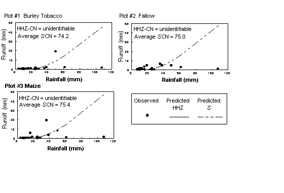
Figure 19. Rainfall-runoff relationships for the four field plots (top) and the three erosion-control plots (bottom) in Chilindamaji Watershed, January � April, 1995. Note that values for the erosion-control plots are significantly lower than those for field plots with the same crop cover.
Because of the short period of record, determining CN using either method may not be reliable and indicative of the catchment response under different crop conditions. A possible method to discriminate among different management practices with respect to their rainfall-runoff relationship in a watershed is to graph P against CN (computed from the running average, as in Table 3), shown in Figure 20. For each of the seven plots, the graph was constructed from the following steps, which are similar to those used in the HHZ-CN approach but without using the P/S>0.456 condition.
Step 1 Arrange the runoff-producing rainfall events in descending order.
Step 2 For each event, compute S from Equation (16).
Step 3 For each event (i), compute a running-average value of S from Equation (35):
 (35)
(35)
where
![]() = the ith event running-average storage parameter,
= the ith event running-average storage parameter,
S
j = the jth event storage parameter,In Equation (35) the following condition must be satisfied:
P
1 > P2 > .... > Pj > .... > Pi(36)(Equation (36) represents the listing of rainfall events in descending order.)
Step 4 Once ![]() is obtained for each event, compute the corresponding
is obtained for each event, compute the corresponding ![]() from Equation (9).
from Equation (9).
Step 5 Finally, graph each rainfall value Pi against the corresponding ![]() .
.
By repeating the same process for each of the seven plots, and graphing P on the x-axis and ![]() on the y-axis, a diagnostic chart is created that can be used to evaluate the effects of different cropping regimes on the catchments' rainfall-runoff relationships. Figure 20, for example, indicates that under similar rainfall conditions, areas planted with maize and managed using traditional methods (solid and open diamonds) produce higher runoff than those areas planted with burley tobacco and managed using traditional conditions (solid and open circles). This difference is greatest for large rainfall events. For smaller rainfall events, however, the response of one of the burley field pits (Pit #1, solid circles) resembled that of both maize plots. Several factors may have contributed to this similarity, among which are the farmers' different land management regimes, soil spatial variability, topography, and rainfall rates. Finally, Figure 20 clearly shows that the three control plots have similar rainfall-runoff relationships, ones characterized by runoff substantially lower than obtained from the field plots, which conclusively demonstrates the effectiveness of erosion-control practices in reducing runoff from fields.
on the y-axis, a diagnostic chart is created that can be used to evaluate the effects of different cropping regimes on the catchments' rainfall-runoff relationships. Figure 20, for example, indicates that under similar rainfall conditions, areas planted with maize and managed using traditional methods (solid and open diamonds) produce higher runoff than those areas planted with burley tobacco and managed using traditional conditions (solid and open circles). This difference is greatest for large rainfall events. For smaller rainfall events, however, the response of one of the burley field pits (Pit #1, solid circles) resembled that of both maize plots. Several factors may have contributed to this similarity, among which are the farmers' different land management regimes, soil spatial variability, topography, and rainfall rates. Finally, Figure 20 clearly shows that the three control plots have similar rainfall-runoff relationships, ones characterized by runoff substantially lower than obtained from the field plots, which conclusively demonstrates the effectiveness of erosion-control practices in reducing runoff from fields.
4.2. Water-Quality Data Analysis
Water-quality data were obtained from the pits following each runoff-producing storm. Samples were collected after stirring the accumulated water in the pits, and sent for laboratory analysis. Results were reported in units of mg/liter.
Mismeasurements and missed measurements of runoff events are the two main causes of reduced sample size. Other problems are the consequences of some extreme rainfall events. On several occasions during the first monitoring season, extreme rainfall events damaged some of the ridges, caused pit overflow, and delayed the process of data collection. Ridge damage is the most problematic for both water quality in general, and for the identification of the impact of management practices on the erosion characteristics of the catchment. Ridge failure caused substantial quantities of sediments to be dislodged, transported, and deposited into collection pits. Such failures must be excluded from the dataset, especially when the catchment area is small, as is the case for the four field plots. There are four reasons for excluding these events from the record:

Figure 20. A comparison of rainfall-runoff relationships between traditional cropping systems and management systems that aim to control erosion. The plot should not be viewed as a predictive tool, but it can be used as a diagnostic tool. Note the significant reduction of runoff as indicated by lower CN values for the same rainfall values associated with the three erosion-control plots. These have near-identical responses, especially under high rainfall conditions � precisely the conditions that produce most of the erosion in traditional management systems.
1. In natural fields, sediments detached from damaged ridges may be deposited on milder slopes prior to reaching the field outlet; sequential ridges or terraces also obstruct sediment transport.
2. Although ridges are integral components of some crop-management systems and must be included in calculations of total soil loss, ridge failure represents a dynamic process that is as much related to soil stability as to soil erosion properties.
3. Given that the contributing areas of the four field plots in Chilindamaji Watershed are delineated by ridges, partial or complete ridge failure is associated with changes in the size of the catchment; consequently, runoff estimates become inconsistent.
4. Most erosion prediction models do not account for ridge failure when calculating the total amount of sediment yield during a fixed period. Instead, the failure process is usually modeled qualitatively, i.e., runoff depth and velocity are calculated from hydraulic equations. If these values exceed ridge tolerance, a failure event is registered. However, these models do not compute the amount of eroded soil.
For this study, we used the following criteria to select an acceptable subset of events for water-quality impact assessment. Table 14 lists all excluded events; Table 15 lists water-quality parameters for all included events.
1. All events for which Q exceeded P were excluded from the sample.
2. Days that were associated with ridge failure on any field or control plot were excluded from the record of all plots. This is necessary to maintain consistency when comparing the water-quality impacts of burley tobacco versus maize. (Note that some of these events, such as Incident 5, produce an extremely high value of soil loss/unit area.)
Table 14. Excluded Runoff Events, Chilindamaji Watershed, Jan. - Apr., 1995
|
Incident |
Month |
Day |
Plot |
Crop |
Soil Loss (kg/ha) |
|
1 |
January |
28 |
1 |
Burley tobacco |
218.92 |
|
2 |
January |
29 |
1 |
Burley tobacco |
Unrecorded/error |
|
3 |
April |
5 |
1 |
Burley tobacco |
1043.11 |
|
4 |
April |
10 |
1 |
Burley tobacco |
3495.00 |
|
5 |
April |
1 |
2 |
Maize |
6470.36 |
|
6 |
March |
3 |
3 |
Maize |
Unrecorded/error |
|
7 |
March |
4 |
3 |
Maize |
Unrecorded/error |
|
8 |
April |
1 |
3 |
Maize |
135.04 |
|
9 |
February |
4 |
M |
Maize |
97.62 |
|
10 |
February |
7 |
M |
Maize |
354.42 |
Table 15. Water-Quality Parameters for Included Events, Chilindamaji Watershed, Jan. - Apr., 1995
TDS: Total dissolved solids (including salts)
SO
4:Oxidized Sulfates (soil, rainfall)NO
3:Nitrate (from soil, rainwater, and fertilizers)SO
4:Orthophosphate (fertilizers)Na:Sodium (soil)
K:Potassium (fertilizers and soil)
Sed.Sediments (i.e., soil loss)
Pit #1 (Burley tobacco)
|
Mon. |
Day |
P |
Q |
pH |
TDS |
SO 4 |
NO 3 |
PO 4 |
Na |
K |
Sed. |
|
mm |
mm |
kg/ha |
kg/ha |
kg/ha |
kg/ha |
kg/ha |
kg/ha |
kg/ha |
|||
|
1 |
7 |
12.4 |
4.49 |
7.5 |
3.65 |
0.56 |
0.0020 |
0.11 |
1.56 |
5.21 |
51.56 |
|
1 |
10 |
50.0 |
33.56 |
7.7 |
136.35 |
4.23 |
0.0070 |
1.46 |
16.41 |
25.52 |
266.15 |
|
2 |
11 |
16.7 |
1.64 |
6.9 |
3.96 |
0.21 |
0.0010 |
0.31 |
2.21 |
4.95 |
41.93 |
|
2 |
14 |
13.3 |
0.39 |
6.9 |
1.18 |
0.54 |
0.0000 |
0.04 |
0.46 |
1.27 |
20.83 |
|
2 |
19 |
12.4 |
2.75 |
7.0 |
5.28 |
0.37 |
0.0010 |
0.11 |
2.43 |
7.29 |
68.06 |
|
2 |
21 |
16.0 |
3.12 |
6.7 |
2.76 |
1.98 |
0.0000 |
0.17 |
2.43 |
7.29 |
117.88 |
|
2 |
25 |
7.0 |
0.75 |
7.2 |
2.38 |
0.10 |
0.0000 |
0.02 |
1.10 |
4.05 |
9.49 |
|
2 |
26 |
5.0 |
1.45 |
6.7 |
1.39 |
0.17 |
0.0000 |
0.05 |
0.52 |
2.60 |
26.74 |
|
2 |
27 |
18.8 |
3.54 |
6.9 |
4.91 |
19.35 |
0.0000 |
0.48 |
1.62 |
6.94 |
27.32 |
|
3 |
27 |
5.8 |
0.24 |
6.9 |
0.79 |
0.12 |
0.0010 |
0.00 |
1.04 |
1.97 |
1.45 |
|
3 |
28 |
5.3 |
0.27 |
6.9 |
0.00 |
0.10 |
0.0010 |
0.00 |
0.64 |
1.27 |
3.7 |
|
4 |
11 |
44.0 |
20.02 |
6.8 |
61.84 |
2.26 |
0.0020 |
0.09 |
5.64 |
9.03 |
48.07 |
|
Total |
206.7 |
72.22 |
n/a |
224.48 |
30.00 |
0.0150 |
2.83 |
36.07 |
77.4 |
683.17 |
|
|
Minimum |
5.0 |
0.24 |
6.7 |
0.00 |
0.10 |
0.0000 |
0.00 |
0.46 |
1.27 |
1.45 |
|
|
Maximum |
50.0 |
33.56 |
7.7 |
136.35 |
19.35 |
0.0070 |
1.46 |
16.41 |
25.52 |
266.15 |
|
|
Average |
17.23 |
6.02 |
7.0 |
18.71 |
2.50 |
0.0013 |
0.24 |
3.01 |
6.45 |
56.93 |
|
Pit #4 (Burley tobacco)
|
Mon. |
Day |
P |
Q |
pH |
TDS |
SO 4 |
NO 3 |
PO 4 |
Na |
K |
Sed. |
|
mm |
mm |
kg/ha |
kg/ha |
kg/ha |
kg/ha |
kg/ha |
kg/ha |
kg/ha |
|||
|
1 |
3 |
25.00 |
2.28 |
6.70 |
14.16 |
0.85 |
0.0000 |
0.01 |
11.17 |
11.93 |
6.06 |
|
1 |
5 |
25.00 |
0.60 |
7.00 |
2.31 |
0.12 |
0.0020 |
0.04 |
4.00 |
8.73 |
26.29 |
|
2 |
8 |
9.50 |
1.95 |
6.90 |
4.09 |
0.24 |
0.0010 |
0.09 |
2.02 |
4.17 |
73.20 |
|
2 |
11 |
16.70 |
0.26 |
7.30 |
2.75 |
0.61 |
0.0030 |
0.06 |
1.39 |
1.89 |
39.25 |
|
2 |
14 |
13.30 |
0.88 |
6.00 |
3.13 |
0.11 |
0.0120 |
0.08 |
1.77 |
2.10 |
48.13 |
|
2 |
19 |
12.40 |
0.94 |
6.70 |
2.46 |
0.24 |
0.0020 |
0.07 |
1.18 |
1.85 |
54.18 |
|
2 |
21 |
16.00 |
4.09 |
8.00 |
5.96 |
0.24 |
0.0000 |
0.18 |
2.02 |
4.54 |
72.19 |
|
3 |
27 |
5.80 |
1.33 |
6.80 |
1.41 |
0.55 |
0.0050 |
0.01 |
2.52 |
2.69 |
9.36 |
|
4 |
2 |
107.50 |
14.57 |
6.90 |
26.50 |
1.68 |
0.0080 |
0.40 |
7.36 |
13.67 |
1076.92 |
|
4 |
8 |
7.20 |
0.41 |
6.60 |
0.45 |
0.07 |
0.0000 |
0.02 |
0.38 |
0.51 |
10.22 |
|
4 |
11 |
44.00 |
0.72 |
6.80 |
0.94 |
2.23 |
0.0030 |
0.26 |
1.68 |
3.03 |
187.79 |
|
4 |
12 |
24.00 |
4.45 |
6.80 |
0.47 |
4.12 |
0.0060 |
0.02 |
3.53 |
5.89 |
197.00 |
|
Total |
306.40 |
32.48 |
n/a |
64.64 |
11.05 |
0.0420 |
1.23 |
39.02 |
61.00 |
1800.58 |
|
|
Minimum |
5.80 |
0.26 |
6.00 |
0.45 |
0.07 |
0.0000 |
0.01 |
0.38 |
0.51 |
6.06 |
|
|
Maximum |
107.50 |
14.57 |
8.00 |
26.50 |
4.12 |
0.0120 |
0.40 |
11.17 |
13.67 |
1076.92 |
|
|
Average |
25.53 |
2.71 |
6.88 |
5.39 |
0.92 |
0.0035 |
0.10 |
3.25 |
5.08 |
150.05 |
|
Pit #2 (Maize)
|
Mon. |
Day |
P |
Q |
pH |
TDS |
SO 4 |
NO 3 |
PO 4 |
Na |
K |
Sed. |
|
mm |
mm |
kg/ha |
kg/ha |
kg/ha |
kg/ha |
kg/ha |
kg/ha |
kg/ha |
|||
|
1 |
3 |
25.00 |
0.20 |
7.10 |
0.53 |
0.12 |
0.0000 |
0.15 |
0.42 |
1.33 |
81.65 |
|
1 |
7 |
12.40 |
0.31 |
8.70 |
3.08 |
0.05 |
0.0000 |
0.05 |
0.93 |
2.26 |
10.57 |
|
1 |
9 |
4.80 |
0.61 |
9.30 |
7.79 |
0.18 |
0.0000 |
0.03 |
3.79 |
4.92 |
65.00 |
|
1 |
10 |
50.00 |
13.71 |
8.90 |
34.28 |
2.61 |
0.0030 |
0.52 |
11.01 |
25.16 |
270.48 |
|
1 |
22 |
12.30 |
0.71 |
9.60 |
11.61 |
0.48 |
0.0000 |
0.08 |
6.51 |
14.06 |
16.09 |
|
2 |
8 |
9.50 |
0.79 |
6.70 |
1.99 |
0.07 |
0.0000 |
0.03 |
0.94 |
1.99 |
18.59 |
|
2 |
17 |
9.00 |
1.25 |
6.70 |
10.00 |
0.14 |
0.0000 |
0.07 |
4.36 |
6.37 |
1.29 |
|
2 |
18 |
2.10 |
1.13 |
6.90 |
0.03 |
0.10 |
0.0000 |
0.01 |
1.75 |
3.39 |
22.38 |
|
2 |
19 |
12.40 |
2.32 |
6.70 |
8.47 |
0.24 |
0.0010 |
0.10 |
3.95 |
7.34 |
58.71 |
|
2 |
21 |
16.00 |
2.58 |
6.80 |
5.87 |
0.23 |
0.0010 |
0.12 |
3.23 |
7.10 |
86.45 |
|
2 |
25 |
7.00 |
0.52 |
7.30 |
1.84 |
0.09 |
0.0000 |
0.01 |
0.89 |
1.86 |
2.42 |
|
2 |
26 |
5.00 |
1.01 |
7.00 |
2.71 |
0.17 |
0.0000 |
0.01 |
1.69 |
4.42 |
3.75 |
|
2 |
27 |
18.80 |
2.47 |
6.30 |
5.36 |
0.25 |
0.0020 |
0.05 |
1.94 |
3.55 |
3.23 |
|
3 |
10 |
9.70 |
1.63 |
6.60 |
4.40 |
0.32 |
0.0000 |
0.05 |
2.02 |
4.03 |
35.08 |
|
3 |
11 |
3.20 |
1.48 |
6.80 |
2.42 |
0.30 |
0.0000 |
0.03 |
0.16 |
2.74 |
3.23 |
|
3 |
14 |
16.00 |
1.77 |
6.70 |
7.60 |
0.24 |
0.0000 |
0.22 |
2.42 |
4.36 |
24.68 |
|
3 |
24 |
10.80 |
1.54 |
6.80 |
1.74 |
0.51 |
0.0000 |
0.01 |
2.37 |
2.77 |
13.34 |
|
3 |
27 |
5.80 |
0.29 |
6.70 |
0.66 |
0.23 |
0.0000 |
0.00 |
0.63 |
0.73 |
3.88 |
|
4 |
2 |
107.50 |
28.73 |
6.40 |
7.94 |
2.91 |
0.0100 |
1.95 |
6.61 |
13.23 |
610.04 |
|
4 |
11 |
44.00 |
7.10 |
6.80 |
7.98 |
0.89 |
0.0090 |
0.12 |
3.55 |
5.77 |
98.91 |
|
4 |
12 |
24.00 |
3.87 |
6.60 |
5.71 |
0.59 |
0.0050 |
0.03 |
2.42 |
3.87 |
17.61 |
|
Total |
405.30 |
74.02 |
n/a |
132.00 |
10.74 |
0.0310 |
3.63 |
61.57 |
121.22 |
1447.37 |
|
|
Minimum |
2.10 |
0.20 |
6.30 |
0.03 |
0.05 |
0.0000 |
0.00 |
0.16 |
0.73 |
1.29 |
|
|
Maximum |
107.50 |
28.73 |
9.60 |
34.28 |
2.91 |
0.0100 |
1.95 |
11.01 |
25.16 |
610.04 |
|
|
Average |
19.30 |
3.52 |
7.21 |
6.29 |
0.51 |
0.0015 |
0.17 |
2.93 |
5.77 |
68.92 |
|
Pit #3 (Maize)
|
Mon. |
Day |
P |
Q |
pH |
TDS |
SO 4 |
NO 3 |
PO 4 |
Na |
K |
Sed. |
|
mm |
mm |
kg/ha |
kg/ha |
kg/ha |
kg/ha |
kg/ha |
kg/ha |
kg/ha |
|||
|
1 |
2 |
28.40 |
1.02 |
7.30 |
1.14 |
1.09 |
0.0000 |
0.07 |
2.60 |
5.68 |
0.57 |
|
1 |
3 |
25.00 |
3.55 |
7.60 |
13.07 |
0.79 |
0.0000 |
0.23 |
17.99 |
40.72 |
12.31 |
|
1 |
4 |
10.80 |
0.44 |
8.80 |
0.19 |
0.44 |
0.0010 |
0.00 |
2.32 |
4.36 |
0.59 |
|
1 |
5 |
25.00 |
0.71 |
8.50 |
1.10 |
0.88 |
0.0000 |
0.04 |
4.36 |
8.33 |
0.34 |
|
1 |
7 |
12.40 |
3.67 |
6.90 |
0.51 |
1.71 |
0.0000 |
0.06 |
2.56 |
4.90 |
0.90 |
|
1 |
9 |
4.80 |
0.72 |
7.90 |
1.02 |
0.48 |
0.0000 |
0.02 |
1.80 |
2.75 |
0.17 |
|
1 |
10 |
50.00 |
16.10 |
7.10 |
53.18 |
2.22 |
0.0040 |
0.61 |
9.23 |
19.39 |
36.93 |
|
1 |
22 |
12.30 |
1.31 |
7.30 |
2.92 |
1.48 |
0.0060 |
0.06 |
4.74 |
9.47 |
0.63 |
|
2 |
11 |
16.70 |
0.16 |
6.20 |
1.50 |
0.23 |
0.0060 |
0.05 |
1.09 |
1.47 |
25.38 |
|
2 |
14 |
13.30 |
1.74 |
6.30 |
0.28 |
0.68 |
0.0010 |
0.07 |
1.54 |
4.03 |
35.18 |
|
2 |
17 |
9.00 |
1.94 |
6.30 |
3.93 |
0.38 |
0.0000 |
0.08 |
3.20 |
5.92 |
22.73 |
|
2 |
19 |
12.40 |
0.83 |
6.30 |
2.36 |
0.23 |
0.0000 |
0.05 |
1.92 |
3.55 |
13.64 |
|
2 |
21 |
16.00 |
5.40 |
7.20 |
6.89 |
0.14 |
0.0010 |
0.49 |
1.23 |
0.00 |
47.40 |
|
2 |
25 |
7.00 |
1.09 |
6.70 |
1.45 |
28.69 |
0.0000 |
0.05 |
0.36 |
1.28 |
26.42 |
|
2 |
26 |
5.00 |
1.18 |
6.10 |
1.85 |
0.17 |
0.0100 |
0.04 |
1.14 |
2.06 |
7.81 |
|
2 |
27 |
18.80 |
5.27 |
6.20 |
7.88 |
0.53 |
0.0030 |
0.19 |
0.15 |
3.69 |
50.47 |
|
3 |
1 |
2.80 |
0.81 |
6.10 |
2.97 |
0.10 |
0.0060 |
0.04 |
0.66 |
1.47 |
30.02 |
|
3 |
10 |
9.70 |
5.22 |
6.50 |
1.36 |
0.68 |
0.0020 |
0.13 |
1.71 |
2.84 |
60.23 |
|
3 |
11 |
3.20 |
0.89 |
6.30 |
1.60 |
0.08 |
0.0030 |
0.10 |
0.26 |
0.83 |
46.46 |
|
3 |
13 |
4.40 |
0.74 |
7.00 |
1.52 |
0.28 |
0.0010 |
0.02 |
0.57 |
0.95 |
7.22 |
|
3 |
14 |
16.00 |
2.41 |
6.50 |
2.73 |
0.95 |
0.0100 |
0.46 |
1.27 |
2.54 |
0.21 |
|
3 |
16 |
8.60 |
1.49 |
6.70 |
2.61 |
0.47 |
0.0000 |
0.02 |
1.14 |
1.42 |
0.09 |
|
3 |
24 |
10.80 |
1.86 |
6.80 |
1.23 |
0.24 |
0.0010 |
0.05 |
1.42 |
3.31 |
29.95 |
|
3 |
27 |
5.80 |
0.67 |
6.80 |
0.95 |
0.23 |
0.0020 |
0.00 |
1.33 |
2.65 |
6.06 |
|
3 |
28 |
5.30 |
2.59 |
6.70 |
1.88 |
0.34 |
0.0030 |
0.05 |
1.42 |
4.69 |
47.44 |
|
4 |
2 |
107.50 |
33.74 |
7.00 |
45.81 |
3.34 |
0.0020 |
0.62 |
5.82 |
13.59 |
250.43 |
|
4 |
3 |
33.00 |
12.64 |
6.60 |
19.03 |
1.42 |
0.0010 |
0.06 |
2.13 |
4.26 |
50.57 |
|
4 |
9 |
2.00 |
0.85 |
6.40 |
1.46 |
0.06 |
0.0000 |
0.00 |
0.14 |
0.38 |
4.05 |
|
4 |
11 |
44.00 |
8.81 |
6.50 |
16.34 |
0.65 |
0.0030 |
0.11 |
1.63 |
4.36 |
57.17 |
|
4 |
12 |
24.00 |
3.12 |
7.10 |
1.71 |
0.38 |
0.0010 |
0.07 |
0.85 |
1.28 |
12.53 |
|
Total |
544.00 |
120.97 |
n/a |
200.46 |
49.34 |
0.0670 |
3.82 |
76.56 |
162.15 |
883.86 |
|
|
Minimum |
2.00 |
0.16 |
6.10 |
0.19 |
0.06 |
0.0000 |
0.00 |
0.14 |
0.00 |
0.09 |
|
|
Maximum |
107.50 |
33.74 |
8.80 |
53.18 |
28.69 |
0.0100 |
0.62 |
17.99 |
40.72 |
250.43 |
|
|
Average |
18.13 |
4.03 |
6.86 |
6.68 |
1.64 |
0.0022 |
0.13 |
2.55 |
5.41 |
29.46 |
|
Control Plot #1 (Burley tobacco)
|
Mon. |
Day |
P |
Q |
pH |
TDS |
SO 4 |
NO 3 |
PO 4 |
Na |
K |
Sed. |
|
mm |
mm |
kg/ha |
kg/ha |
kg/ha |
kg/ha |
kg/ha |
kg/ha |
kg/ha |
|||
|
1 |
3 |
25.00 |
1.30 |
7.30 |
11.56 |
0.29 |
0.0010 |
0.03 |
4.68 |
9.18 |
7.20 |
|
2 |
11 |
16.70 |
0.27 |
7.00 |
0.53 |
0.11 |
0.0020 |
0.01 |
1.56 |
1.29 |
13.26 |
|
2 |
14 |
13.30 |
0.23 |
7.10 |
1.13 |
0.22 |
0.0000 |
0.02 |
1.08 |
1.05 |
9.05 |
|
2 |
17 |
9.00 |
0.12 |
7.00 |
0.86 |
0.08 |
0.0000 |
0.01 |
1.05 |
0.95 |
4.17 |
|
2 |
19 |
12.40 |
0.35 |
6.80 |
2.35 |
0.13 |
0.0010 |
0.01 |
1.11 |
1.20 |
9.66 |
|
2 |
21 |
16.00 |
0.58 |
6.60 |
2.54 |
0.31 |
0.0010 |
0.05 |
1.04 |
1.08 |
24.30 |
|
2 |
27 |
18.80 |
1.02 |
6.90 |
4.68 |
0.50 |
0.0010 |
0.05 |
1.96 |
1.89 |
30.52 |
|
3 |
10 |
9.70 |
0.81 |
6.80 |
1.24 |
0.14 |
0.0000 |
0.01 |
0.70 |
0.90 |
4.60 |
|
3 |
14 |
16.00 |
0.28 |
6.80 |
0.41 |
0.10 |
0.0000 |
0.00 |
1.08 |
0.96 |
2.64 |
|
3 |
24 |
10.80 |
0.18 |
6.80 |
0.20 |
0.07 |
0.0010 |
0.00 |
1.08 |
1.34 |
0.09 |
|
4 |
12 |
24.00 |
0.32 |
6.90 |
1.10 |
0.09 |
0.0000 |
0.02 |
0.28 |
0.32 |
12.72 |
|
Total |
171.70 |
5.46 |
n/a |
26.59 |
2.05 |
0.0070 |
0.21 |
15.61 |
20.16 |
118.21 |
|
|
Minimum |
9.00 |
0.12 |
6.60 |
0.20 |
0.07 |
0.0000 |
0.00 |
0.28 |
0.32 |
0.09 |
|
|
Maximum |
25.00 |
1.30 |
7.30 |
11.56 |
0.50 |
0.0020 |
0.05 |
4.68 |
9.18 |
30.52 |
|
|
Average |
15.61 |
0.50 |
6.91 |
2.42 |
0.19 |
0.0006 |
0.02 |
1.42 |
1.83 |
10.75 |
|
Control Plot #2 (Fallow)
|
Mon. |
Day |
P |
Q |
pH |
TDS |
SO 4 |
NO 3 |
PO 4 |
Na |
K |
Sed. |
|
mm |
mm |
kg/ha |
kg/ha |
kg/ha |
kg/ha |
kg/ha |
kg/ha |
kg/ha |
|||
|
1 |
3 |
25.00 |
1.70 |
7.60 |
10.74 |
0.32 |
0.0000 |
0.02 |
6.16 |
6.27 |
39.82 |
|
1 |
5 |
25.00 |
0.10 |
7.20 |
1.38 |
0.07 |
0.0000 |
0.02 |
0.84 |
1.41 |
3.48 |
|
2 |
8 |
9.50 |
1.41 |
7.20 |
7.23 |
0.36 |
0.0030 |
0.12 |
4.16 |
3.60 |
22.40 |
|
2 |
11 |
16.70 |
0.17 |
6.50 |
0.77 |
0.07 |
0.0010 |
0.01 |
0.25 |
0.50 |
5.45 |
|
2 |
14 |
13.30 |
0.73 |
7.00 |
0.68 |
0.47 |
0.0010 |
0.02 |
1.20 |
1.30 |
30.10 |
|
2 |
17 |
9.00 |
0.12 |
6.80 |
0.01 |
0.11 |
0.0000 |
0.01 |
0.83 |
0.60 |
3.93 |
|
2 |
19 |
12.40 |
1.35 |
6.70 |
3.55 |
0.00 |
0.0020 |
0.07 |
0.96 |
1.20 |
28.00 |
|
2 |
21 |
16.00 |
3.28 |
6.80 |
2.38 |
1.67 |
0.0000 |
0.09 |
1.62 |
2.16 |
33.12 |
|
4 |
12 |
24.00 |
0.72 |
6.90 |
0.65 |
0.10 |
0.0000 |
0.01 |
0.42 |
0.66 |
5.02 |
|
Total |
150.90 |
9.58 |
n/a |
27.38 |
3.16 |
0.0070 |
0.38 |
16.44 |
17.70 |
171.32 |
|
|
Minimum |
9.00 |
0.10 |
6.50 |
0.01 |
0.00 |
0.0000 |
0.01 |
0.25 |
0.50 |
3.48 |
|
|
Maximum |
25.00 |
3.28 |
7.60 |
10.74 |
1.67 |
0.0030 |
0.12 |
6.16 |
6.27 |
39.82 |
|
|
Average |
16.77 |
1.06 |
6.97 |
3.04 |
0.35 |
0.0008 |
0.04 |
1.83 |
1.97 |
19.04 |
|
Control Plot #3 (Maize)
|
Mon. |
Day |
P |
Q |
pH |
TDS |
SO 4 |
NO 3 |
PO 4 |
Na |
K |
Sed. |
|
mm |
mm |
kg/ha |
kg/ha |
kg/ha |
kg/ha |
kg/ha |
kg/ha |
kg/ha |
|||
|
1 |
3 |
25.00 |
1.30 |
8.40 |
6.84 |
0.45 |
0.0010 |
0.09 |
6.12 |
5.94 |
17.28 |
|
1 |
5 |
25.00 |
0.02 |
8.30 |
3.15 |
0.14 |
0.0000 |
0.01 |
2.55 |
2.26 |
1.87 |
|
2 |
11 |
16.70 |
0.27 |
6.90 |
2.40 |
0.07 |
0.0000 |
0.01 |
1.50 |
1.20 |
2.16 |
|
2 |
14 |
13.30 |
0.33 |
6.40 |
1.33 |
0.09 |
0.0040 |
0.03 |
1.56 |
1.35 |
12.18 |
|
2 |
17 |
9.00 |
0.02 |
7.00 |
0.50 |
0.04 |
0.0000 |
0.00 |
0.71 |
0.63 |
1.62 |
|
2 |
19 |
12.40 |
0.35 |
6.80 |
1.88 |
0.18 |
0.0010 |
0.03 |
1.20 |
1.20 |
16.50 |
|
2 |
21 |
16.00 |
5.48 |
5.70 |
17.75 |
0.05 |
0.0530 |
0.47 |
2.03 |
2.90 |
138.62 |
|
2 |
27 |
18.80 |
1.42 |
7.00 |
5.15 |
0.83 |
0.0000 |
0.05 |
1.89 |
2.07 |
31.14 |
|
3 |
14 |
16.00 |
0.28 |
6.70 |
0.83 |
0.08 |
0.0010 |
0.01 |
0.87 |
1.08 |
1.26 |
|
3 |
24 |
10.80 |
0.38 |
6.40 |
0.44 |
0.10 |
0.0010 |
0.04 |
1.68 |
2.16 |
0.76 |
|
4 |
12 |
24.00 |
0.52 |
7.30 |
6.64 |
0.02 |
0.0000 |
0.01 |
0.40 |
0.60 |
7.50 |
|
Total |
187.00 |
10.37 |
n/a |
46.92 |
2.05 |
0.0610 |
0.74 |
20.51 |
21.39 |
230.89 |
|
|
Minimum |
9.00 |
0.02 |
5.70 |
0.44 |
0.02 |
0.0000 |
0.00 |
0.40 |
0.60 |
0.76 |
|
|
Maximum |
25.00 |
5.48 |
8.40 |
17.75 |
0.83 |
0.0530 |
0.47 |
6.12 |
5.94 |
138.62 |
|
|
Average |
17.00 |
0.94 |
6.99 |
4.27 |
0.19 |
0.0055 |
0.07 |
1.86 |
1.94 |
20.99 |
|
Because the available record consists of a single monitoring season, statistical analysis of the data beyond total values would lack the required level of significance. At the current stage of the monitoring efforts, therefore, we will use total values of water-quality variables to discriminate between the two management crops and the corresponding traditional versus soil-conservation practices. In the following section, we will (a) consider each of the water-quality parameters, and (b) intercompare observed values from each of the sampling locations.
4.2.2. A Comparison of Crops and Crop Management Practices
4.2.2.1. Total Dissolved Solids (TDS)
Total dissolved solids include the inorganic salts such as calcium, Ca, magnesium, Mg, and sodium, Na. The presence of large amounts of these salts in runoff indicates high soil salinity. Although Ca does not constitute direct harm, its presence in high concentrations leads to increased salinity of both surface water and groundwater. The presence of Ca in abundance is common because it is a major constituent of several mineral rocks and soils. In general, Ca can be found in runoff water with pH values from 7 to 8, a range close to many runoff events in the watershed. Acceptable limits for Ca concentration are usually based on determinations of adverse impact at the runoff's end-point, or on agreed-upon levels of salts ultimately leaching to groundwater.
Figure 21 and the accompanying table indicate total monthly and seasonal TDS values from the experimental locations in Chilindamaji Watershed. Note that the amount of TDS in surface runoff from the field plots is almost an order of magnitude higher than comparable losses from the control plots. Fallow land has the same order of TDS losses as do the two cropped control plots.

Figure 21. Monthly and seasonal TDS losses from field and erosion-control plots in Chilindamaji Watershed.
4.2.2.2. Oxidized Sulfate (SO4)
The same processes that govern the presence of Ca in natural waters control concentrations of SO4. Furthermore, SO4 occurs in rainfall at concentrations that vary with the level of air pollution (causing the "Acid Rain" problem in industrialized countries). Under unpolluted conditions, rainwater SO4 concentrations of around 1.0 mg/l are normal. A concentration as high as 250 mg/l is acceptable even for drinking water. Figure 22 and the accompanying table indicate total monthly and seasonal SO4 losses from the experimental locations in Chilindamaji Watershed. Note that the concentration of SO4 in surface runoff from the field plots is almost an order of magnitude higher than comparable losses from the control plots. Fallow land loses SO4 in concentrations similar to those of the two cropped control plots.

Figure 22. Monthly and seasonal SO4 losses from field and erosion-control plots in Chilindamaji Watershed.
As mentioned in Section 2.2.4, NO3 is but one of the many forms nitrogen assumes in nature. Unlike ammonium and orthophosphate, nitrate adsorption by soil particles is very low. Thus, the amount of NO3 transported by runoff is not significant. Infiltration below the surface and to the groundwater aquifer is the fate of most soil NO3. In surface waters, NO3 concentrations can increase when previously infiltrated water resurfaces as baseflow.
The physical processes controlling the infiltration rate also control the rate of denitrification (the process of converting ammonia [NH4] into nitrite [NO2] and then to NO3: Frere and Leonard, 1982). In sum, therefore, only low concentrations of NO3 are lost in sediment and runoff. However, note that NO3 concentrations alone do not reflect the full spectrum of nitrogen losses from the surface soil. Figure 23 and the accompanying table indicate total monthly and seasonal NO3 losses from the experimental locations in Chilindamaji Watershed. Clearly, NO3 losses in the maize field and erosion-control plots are roughly equal, demonstrating that soil loss itself does not account for the observed NO3 concentrations, i.e., NO3 loss in sediment is less than NO3 loss due to infiltration. Again, note that organic forms of nitrogen, which may be present with washed-off fertilizers, are unmeasured and may be significantly high.

Figure 23. Monthly and seasonal NO3 losses from field and erosion-control plots in Chilindamaji Watershed.
As does NO3, PO4 originates from a complex phosphorous cycle that involves both the decomposition of plants and the application of fertilizers. The similarity ends here, since PO4 has a high desorption rate by soil particles. Much higher magnitudes of PO4 are therefore present in surface waters. PO4 is a primary cause of eutrophification, one of the major problems facing surface water bodies. Figure 24 and the accompanying table indicate total monthly and seasonal PO4 losses from the experimental locations in Chilindamaji Watershed. The figure indicates that higher rates of PO4 losses may be expected from maize fields than from tobacco or fallow fields, regardless of whether traditional or soil-conserving practices are used. These higher rates can be attributed to higher sediment yields (see Section 4.2.2.6) as well as to different cultural practices and fertilizer-management regimes.

Figure 24. Monthly and seasonal PO4 losses from field and erosion-control plots in Chilindamaji Watershed.
4.2.2.5. Other dissolved salts: Sodium (Na) and Potassium (K)
Both Na and K occur naturally in minerals and clay particles. While relatively high Na concentrations in surface water usually has minimal adverse impacts on aquatic habitats and humans, high concentrations of K is lethal to several species of freshwater fish and, in potable water, can damage human health. High concentrations of K can be found in nutrient-enriched waters and in eutrophic water bodies.
K is an essential element for proper crop growth, and in some cases K-deficient soils are augmented by fertilizers. Figures 25 and 26 and the accompanying tables demonstrate the effects of crop type and management practices on the presence of Na and K in surface water. For both elements, maize farming produced higher losses than from fallow fields or from tobacco farming.

Figure 25. Monthly and seasonal Na losses from field and erosion-control plots in Chilindamaji Watershed.

Figure 26. Monthly and seasonal K losses from field and erosion-control plots in Chilindamaji Watershed.
Excluded events (Section 4.2.1) lead to a large underestimation of the total seasonal sediment yield from the microcatchments. Numerical values of sediment yield based on the filtered sample cannot be used, therefore, to indicate the absolute magnitude of soil losses. Values of sediment loss can be used only in a relative context, i.e., for comparing farming methods and crops under similar conditions. To illustrate the loss of information due to sample filtering, we calculated monthly and seasonal sediment losses based on (a) the partial elimination method, in which events were discarded only with respect to the plot(s) affected (Figure 27), and (b) the completely filtered sample, in which an excluded event for any one plot resulted in discarding that event for all plots (Figure 28).

Figure 27. Sediment yields based on the partial elimination method. Note the large values of soil loss during the month of January (the month of ridge construction) from the erosion-control plots. Excessive soil loss may occur from unfinished ridges, yet will not be reported as ridge failure or damage.

Figure 28. Sediment yields based on the filtered sample. Note that under normal conditions (i.e., severe storms causing ridge damage on at least one plot were discarded), erosion-control plots have much lower soil losses than do plots cultivated under traditional agricultural methods. Furthermore, notice the substantial amount of soil loss observed from pit 4 during April.
In comparing Figures 27 and 28, it is clear that the filtered sample (Figure 28), although necessary for reliable intercomparisons, represents a gross underestimation of the total seasonal sediment yield. Large rainfall events can cause ridge damage and excessive surface erosion on one plot, simultaneously affecting other plots but less destructively. In fact, these events are the most crucial in understanding the field response to rainfall. The impact of these events is clear from Figure 27. If judgment is to be made based on the filtered sample (Figure 28), the wrong conclusion may be drawn, i.e., "Although erosion-control plots have reduced the erosion rates, erosion was not that significant of a problem to start with." Figure 27 demonstrates that such a statement does not reflect reality.
5. A Simple Method for Multiple-Objective Evaluation (MOE)
Sustainable agricultural development requires regulating the impacts of agricultural activities on several variables. For example, it is in the interest of the farmer to maximize crop yields while minimizing soil and fertilizer losses due to erosion. Concurrently, it is in the interest of society as a whole to eradicate or minimize the presence of harmful chemicals in surface waters. Considering these sometimes competing interests in a MOE is a complex task, one that requires input from social and physical scientists who are experts in anthropology, agronomy, climatology and hydrology, economics, and other disciplines. To add to its inherent complexity, MOE involves consideration of variables that do not necessarily share common units and do not reflect similar processes. For example, when determining an aggregate measure of performance, soil loss cannot be added to nitrate loss, regardless of the fact that both have units of kg/ha.
There are many approaches for evaluating management alternatives when faced with competing decision variables. Decision variables are those factors or effects in a MOE that must be maximized (e.g., farm profits) or minimized (e.g., soil losses). One approach is that of the USDA, which has developed a multiple-objective decision-support system for farm water-quality management (WQDSS; Yakowitz et al, 1993, Imam, 1994). WQDSS uses simulation and decision models to rank different farm-management systems based on their impacts on water quality as well as their effects on farm profitability. However, WQDSS requires much data in order to parameterize its simulation modules, and it also requires users to be familiar with decision theory. For MEMP's current needs, therefore, we advocate and propose a simple approach to MOE. We caution, however, that while this simple MOE can be used diagnostically, it should not be used as a stand-alone decisionmaking tool.
Most MOE methods are based on transforming the assembly of variables into common indicators, scores, or ranks that can be summed to obtain an aggregate measure of performance associated with competing alternatives. These aggregate measures are then compared against each other to determine the alternative that appears to satisfy most of the policy issues. Our proposed MOE framework is based on minimizing a summed value of ranks. For each decision variable (soil loss, nitrate loss, profit, crop yield, etc.), we assign a rank to each alternative (i.e., crop type and farm-management system) based on its relative performance against all other alternatives. If a decision variable is to be minimized, alternatives are ranked by integer values that increase as the decision variable associated with the alternative increases. Conversely, if a decision variable is to be maximized, alternatives are ranked by integer values that decrease as the decision variable associated with the alternative increases. For example, consider the seven plots in Chilindamaji Watershed. The seasonal totals of all seven water-quality indicators (the decision variables TDS, SO
4, NO3, PO4, Na, K, Sed.), must be minimized. (Conversely, if crop yield or sales profit data were available, then these would be maximized.) Table 16 illustrates this approach for the Chilindamaji case study, and is to be read as follows:Step 1 For each row (rows are the decision variables), identify the alternative that has the lowest (if minimized) or the highest (if maximized) value. Assign a rank of 1 to this alternative in the row.
Step 2 Repeat the process in the same row; find the alternative associated with the next lowest (or highest) value, assign the rank 2. Repeat the process until all ranks are assigned within the row.
Step 3 Repeat Steps 1 and 2 for each row (i.e., for each decision variable).
Step 4 Once all alternatives for each decision variable are assigned ranks, sum all ranks in each column.
Step 5 The alternative that has the lowest sum of ranks is the "best" alternative.
Note: If two alternatives have the same value for a decision variable, use subjectivity to determine which gets the lower rank. Use similar subjectivity in case of a tie in the sum of ranks.
Table 16. Demonstration of a Simple MOE for the Chilindamaji Watershed
|
Direction of assigning a rank to each alternative with respect to each decision variable: |
|||||||||||||||
|
Rule 1: |
If maximizing the variable, the alternative with the highest value is assigned the lowest rank. |
||||||||||||||
|
Rule 2: |
If minimizing the variable, the alternative with the lowest value is assigned the lowest rank. |
||||||||||||||
|
Alternatives |
|||||||||||||||
|
Decision Variable |
Direction |
Pit 1 (Burley) |
Pit 2 (Maize) |
Pit 3 (Maize) |
Pit 4 (Burley) |
Plot 1 (Burley) |
Plot 2 (Fallow) |
Plot 3 (Maize) |
|||||||
|
Value |
Rank |
Value |
Rank |
Value |
Rank |
Value |
Rank |
Value |
Rank |
Value |
Rank |
Value |
Rank |
||
|
TDS |
Minimize |
224.48 |
7 |
132 |
5 |
200.46 |
6 |
64.64 |
4 |
26.59 |
1 |
27.38 |
2 |
46.92 |
3 |
|
SO 4 |
Minimize |
30.00 |
6 |
10.74 |
4 |
49.34 |
7 |
11.05 |
5 |
2.05 |
1 |
3.16 |
3 |
2.05 |
2 |
|
NO 3 |
Minimize |
0.02 |
3 |
0.03 |
4 |
0.07 |
7 |
0.04 |
5 |
0.01 |
1 |
0.01 |
2 |
0.06 |
6 |
|
PO 4 |
Minimize |
2.83 |
5 |
3.63 |
6 |
3.82 |
7 |
1.23 |
4 |
0.21 |
1 |
0.38 |
2 |
0.74 |
3 |
|
Na |
Minimize |
36.07 |
4 |
61.57 |
6 |
76.56 |
7 |
39.02 |
5 |
15.61 |
1 |
16.44 |
2 |
20.51 |
3 |
|
K |
Minimize |
77.40 |
5 |
121.22 |
6 |
162.15 |
7 |
61 |
4 |
20.16 |
2 |
17.7 |
1 |
21.39 |
3 |
|
Sed. |
Minimize |
683.17 |
4 |
1447.37 |
6 |
883.86 |
5 |
1800.58 |
7 |
118.21 |
1 |
171.32 |
2 |
230.89 |
3 |
|
Sum of ranks from each column |
34 |
37 |
46 |
34 |
8 |
14 |
23 |
||||||||
|
FINAL RANK |
4 |
6 |
7 |
5 |
1 |
2 |
3 |
||||||||
Monitoring activities that are designed to identify causes and effects of specific environmental problems differ from programs designed to inventory environmental resources. Building a successful environmental and water-quality monitoring program requires a clear vision of the environmental problem being addressed, a set of clearly stated and defined goals and objectives for the monitoring activities, and a well-defined criterion that can be used to judge whether these objectives have been achieved. Additionally, monitoring programs that are designed for the purpose of identifying parameters required in simulation studies are usually problem-focused, site-specific, and model-dependent. In the final analysis, these issues must be considered when designing monitoring and sampling schemes.
The concept of "representativeness" is an important aspect of water-quality monitoring. Statistical or analytical inferences concerning the impact of human activities on water quality may be confounded by the effects of topography, soil, and other factors. This is the fundamental reason for collecting data from several locations. In fact, the larger the number of variables (i.e., soil, topography, slope, etc.), the larger the number of sample sites required in order to adequately analyze and categorize the impact of these variables.
"Scaling" is another important aspect of water-quality monitoring. Scale effects must be considered when determining the representativeness of sampling locations. For example, consider soil-loss data collected from a small microcatchment with uniform slope. Although the microcatchment may be representative of the dominant soil and crop management regimes at larger scales, it may not reflect the effects of large-scale topographic control of soil erosion. Intervening processes (such as deposition) govern sediment transport from the watershed at these larger scales.
Ensuring the usefulness of data is extremely important. Monitoring agencies must guard against problems that can affect the reliability of the collected record. Data quality control can be attained through the following guidelines:
1. Consistency: Consistent methods must be used when collecting samples. Factors that are considered constant for the duration of the experiment should remain constant throughout. One example is the contributing area of a microcatchment. If such factors cannot be held constant, their variability must be monitored and reported.
2. Replicability: When collecting water-quality samples, more than one sample must be sent to the laboratory. The collection of more than one sample, especially when these samples are separated in time, provides a guard against errors and random noise that can contaminate a single sample.
3. Timely reporting: This is extremely important when sample collection is performed by individuals other than those performing or documenting the analysis. Reporting analytical results promptly will (a) enable the tracking of problems as they occur, and (b) provide an opportunity to assure the integrity of the data samples.
4. Reliability: Predetermined guidelines can be established to determine whether the numerical values reported correspond with the physical and conceptual notions underlying the experiment. For example, runoff values must be less than rainfall when baseflow is not expected to contribute to the collected runoff. Reliability guidelines must be simple and easy to perform so that MEMP staff can perform these checks easily and unequivocally.
5. Documentation accuracy: Raw data, procedures, and results must be documented fully and accurately. A knowledgeable supervisor must critically read the staff's reports; he or she must check for and correct any lapses or errors.
Our assessment of MEMP's first year of activities in Chilindamaji indicates that the program satisfies several components of a successful monitoring program. However, there are some aspects of the program that can be substantially improved with minimal or no costs, but which do require some effort on the part of MEMP staff, collaborating local farmers, and MEMP's outside experts. In Section 6.1 to 6.3, we offer several recommendations, separated into three subcategories: Recommendations regarding experimental infrastructure, recommendations regarding data reporting and documentation, and future directions.
6.1. Recommendations Regarding Experimental Infrastructure
The following recommendations will result in a substantial improvement in the reliability and accuracy of the collected rainfall-runoff data.
Actions must be taken during future data-collection seasons to ensure that water collected in each pit represents the surface runoff. Errors due to direct rainfall and the inclusion of baseflow must be minimized by covering the pits and securing the impermeability of their lining. Pit covers can be designed to allow for runoff measurements and water-quality sampling while being immune to damage or theft. The installation of handpumps will facilitate the cleaning and preparation of pits for future rain events.
Under ideal conditions, the contributing area of each microcatchment must remain constant during the experiment through the use of boundaries impermeable to damage by extreme events. This is harder to attain in the field than in theory, and consequently evaluations of the total contributing area must be made when ridges fail. Subsets of contributing areas can be predetermined, the smallest of which represents the microcatchment itself. Larger areas include the microcatchment and, progressively, the areas beyond the ridges. Whenever a ridge failure occurs, the contributing area associated with this event can then immediately be adjusted to reflect the larger microcatchment. If the damaged ridges subsequently remain unrepaired, the larger area must become the contributing area to the pit from that point on. Farmers should therefore be encouraged to maintain ridges on their fields in good condition for their own well-being as well as for areal consistency throughout the experiment.
Under ideal conditions, each microcatchment must be equipped with its own raingage. It is not essential to install a sophisticated raingage. Standard, nonrecording, simple, yet inexpensive cumulative precipitation gages can be installed at the manufacturer's recommended height above or adjacent to the collection pit. Individual raingages for each pit are preferable because most large rainfall events are characterized by the significant spatial variability common to monsoon-type tropical storms. The distances between the field microcatchments are large enough to justify individual raingages.
The amount of soil loss during a single rainfall event correlates more strongly with the maximum intensity of the storm than with total rainfall. By providing rainfall intensity data, a better understanding of the rainfall-erosion relationship for each of the sampling locations can be ascertained. So as to achieve this purpose, it is preferable to have an intensity record at each pit. However, the cost associated with installing, maintaining, and operating additional recording raingages may be prohibitive.
6.2. Recommendations Regarding Data, Reporting, and Documentation
6.2.1. Nutrient Application Data
Knowledge of the timing of nutrient applications is not sufficient to describe a farm-management regime, nor is it sufficient to evaluate the impact of the regime on water quality. Documentation of the amount and type of applied fertilizer, as well as the method of application, is also necessary.
6.2.2. Full Reporting of Rainfall Events
Although rainfall events that do not produce runoff cannot be used to determine the hydrologic response of catchments, knowledge of these events is helpful in identifying the overall hydrologic characteristics of the watershed. Furthermore, as an integral part of the water-quality data and from a statistical perspective, it is important to report these events.
Soil texture classifications were made for some sediment samples in January, 1995. Although soil texture is useful in understanding the sedimentation process, it must be complemented by particle-size distribution data from the soil on the field. Ideally, primary particle-size distributions (i.e., percents of sand, silt, and clay) should be determined at several depths along a full root zone profile for each crop. These data will aid in determining the water-retention properties of the soils.
6.2.4. Promptness, Initial Analysis, and Feedback
As discussed above, prompt collection and reporting of rainfall-runoff events will allow MEMP staff to perform initial data assessments. If errors are found to exist, a feedback communication must be initiated, and the conditions associated with the error must be noted and rectified if possible.
It must recognized that because of external controlling and influencing factors (climate variability and farm prices being an example of each), environmental monitoring and impact assessment programs designed to provide recommendations to policymakers must be both comprehensive and long-term. It is counterproductive to terminate such programs after one or two data-collection seasons. From a scientific perspective, such a short duration does not provide a statistically robust record. Conversely, a record that is statistically significant provides much greater confidence in the results, clearly an important objective when the results are meant to be used as policy guidelines. A commonly shared objective of any environmental monitoring program is the reduction of uncertainties associated with decisionmaking. This can only be achieved by monitoring land and water-quality responses under a variety of conditions, especially those that occur as a result of the normal interannual variability of climate.
Agricultural models such as the USLE can be used to predict the impact of farm operations on water quality. However, these predictive tools require fitting to local conditions (refer to Section 2.2.3 and the nonrepresentativeness of Table 11 to conditions in Malawi). A longer record will permit scientists to calibrate models such as the USLE for both normal and extreme climate conditions in Malawi.
Foster, G.R., McCool D.K., Renard K.G., and W.C. Moldenhauer, 1981. Conversion of the universal soil loss equation to SI metric units. Journal of Soil and Water Conservation, 36:6.
Foster, G.R., 1982. Modeling the Erosion Process. In: T.C. Haan (ed.), Hydrologic Modeling of Small Watersheds. St. Joseph, MI: American Society of Agricultural Engineers, 297-380.
Frere, M.H. and Leonard R.A., 1982. Modeling the Quality of Water from Agricultural Land. In: T.C. Haan (ed.), Hydrologic Modeling of Small Watersheds. St. Joseph, MI: American Society of Agricultural Engineers, 381-405.
Hawkins, R.H., 1978.
Effects of rainfall intensity on runoff curve number. Hydrology and Water Resources of Arizona and the Southwest 8, 53-64.Hawkins, R.H., 1993. Asymptotic determination of runoff curve numbers from data. Journal of Irrigation and Drainage Engineering 119:2, 334-345.
Hawkins, R.H., A.T. Hejlmfelt, and A.W. Zevenburgen, 1985. Runoff probability, storm depth, and curve numbers. Journal of Irrigation and Drainage Engineering 111:4, 330-340.
Hejlmfelt, A.T., 1980. Empirical investigation of curve number technique. Journal of Hydraulic Division 106:HY9, 1471-1476.
Imam, B. 1994. Nonlinear Uncertainty Analysis of Multiple Criteria Natural Resource Decision Support Systems. Ph.D. dissertation, School of Renewable Natural Resources, The University of Arizona, 382 pp.
Knisel, W.G. 1993. GLEAMS II. Groundwater Loading Effects from Agricultural Management Systems, User Manual. Washington, D.C.: U.S. Department of Agriculture, Agricultural Research Service (available in electronic form).
McCool, D.K., L.C. Brown, G.R. Foster, C.K. Mutchler, and L.D. Meyer, 1987. Revised slope steepness factor for the Universal Soil Loss Equation. Transactions of the American Society of Agricultural Engineers 32:1378-1396.
McCool, D.K., G.R. Foster, C.K. Mutchler, and L.D. Meyer, 1989. Revised slope length factor for the Universal Soil Loss Equation. Transactions of the American Society of Agricultural Engineers 32:1571-1576.
Mokhothu, N.M., 1994. Field and Catchment Water and Soil Monitoring. MEMP Internal Report.
Mutchler, C.K., C.E. Murphree, and K.C. McGregor, 1982. Subfactor method for computing C-factor for continuous cotton. Transactions of the American Society of Agricultural Engineers 25:327-332.
Pimentel et al, 1995. Environmental and economic costs of soil erosion and conservation benefits. Science 267, 1211-1237.
Ponce, V.M. and R.H. Hawkins, 1996. Runoff Curve Number: Has It Reached Maturity? Journal of Hydrologic Engineering, 1:1.
Renard, K.G. (ed.), 1992. Predicting Soil Erosion by Water - A Guide to Conservation Planning with the Revised Universal Soil Loss Equation (RUSLE). Washington, D.C.: U.S. Department of Agriculture, Agricultural Research Service, 354 pp.
U.S. Soil and Conservation Service, 1985. National Engineering Handbook, Section 4: Hydrology. Washington, D.C.: U.S. Department of Agriculture.
Williams, J.R., C.A. Jones, and P.T. Dyke, 1990. The EPIC Model. In: A.N. Sharpley and J.R. Williams (eds.). EPIC - Erosion Productivity Impact Calculator: 1. Model Documentation. Washington, D.C.: U.S. Department of Agriculture Technical Bulletin No. 1768.
Wischmeier, W.H. and D.D. Smith, 1978. Predicting Rainfall Erosion Losses - A Guide to Conservation Planning. Washington, D.C.: U.S. Department of Agriculture, Agriculture Handbook No. 537, 57 pp.